【笔记】动手学深度学习v2(全73讲)李沐
发布时间 : 2023-09-30 13:11
阅读 :
00预告 学习深度学习关键是动手
01课程安排 目标
介绍深度学习经典和最新模型
LeNet, ResNet, LSTM, BERT, …
机器学习
实践
使用Pytorch实现介绍的知识点
在真实数据上体验算法效果
内容
深度学习基础——线性神经网络,多层感知机
卷积神经网络——LeNet, AlexNet, VGG, Inception, ResNet
循环神经网络——RNN, GRU, LSTM, seq2seq
注意力机制——Attention, Transformer
优化算法——SGD, Momentum, Adam
高性能计算——并行,多GPU,分布式
计算机视觉——目标检测,语义分割
自然语言处理——词嵌入,BERT
你将学到什么
资源
02深度学习介绍 03安装 pip install d2l -i http://pypi.douban.com/simple –trusted-host pypi.douban.com –user
05线性代数 代码 标量由只有一个元素的张量表示
1
2
3
4
5
6
import torch x = torch.tensor([3.0]) y = torch.tensor([2.0]) x + y, x * y, x / y, x**y
你可以将向量视为标量值组成的列表
通过张量的索引来访问任一元素
06矩阵计算 07 自动求导 08线性回归 + 基础优化算法 线性回归
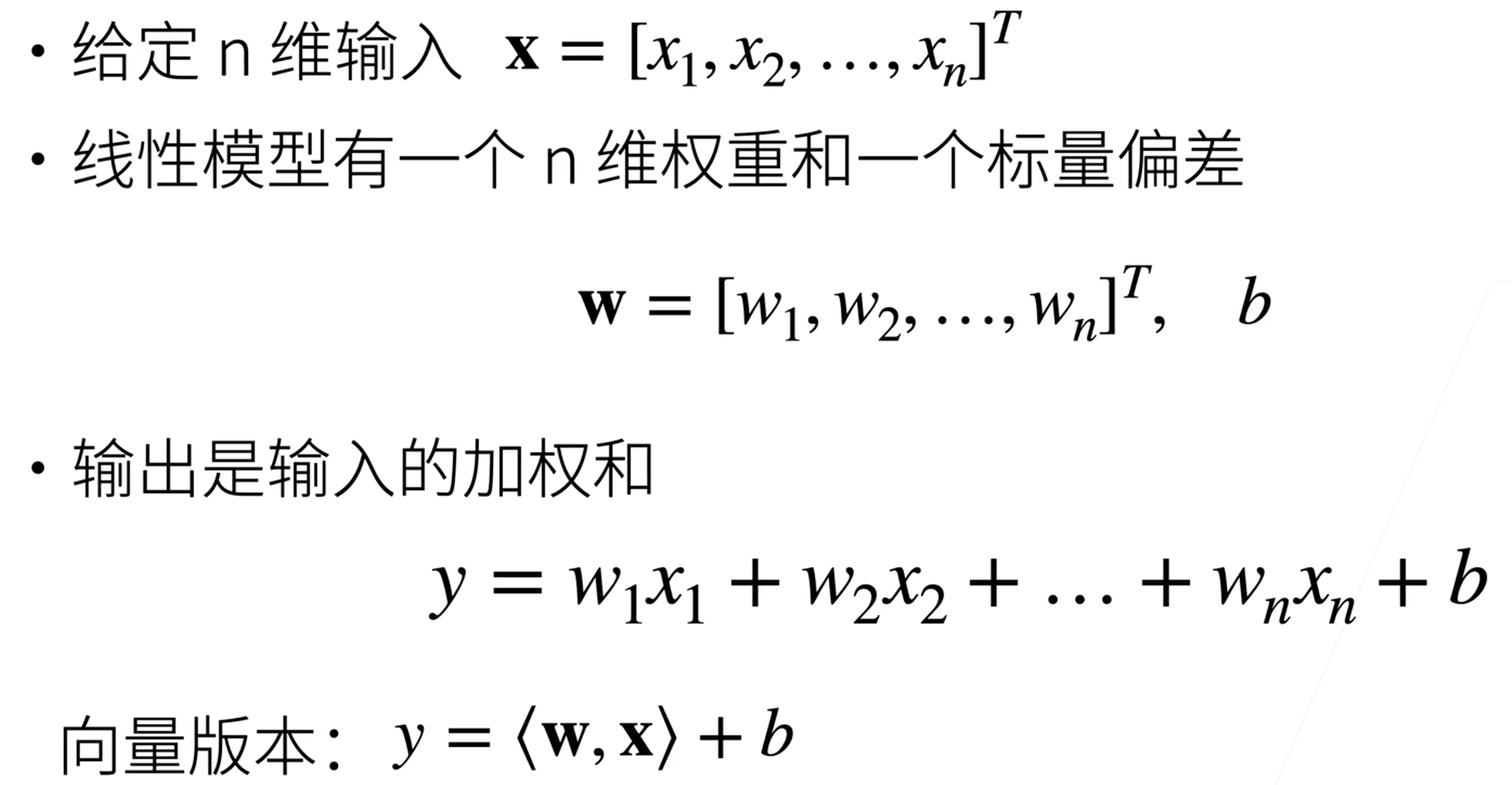
一个简化模型 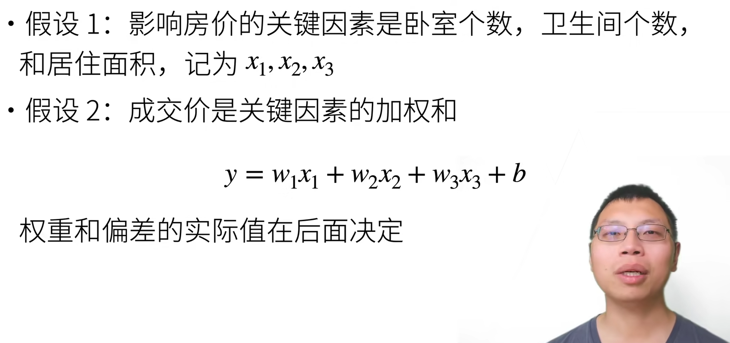
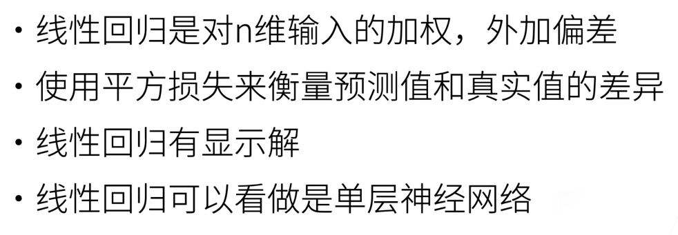
线性模型
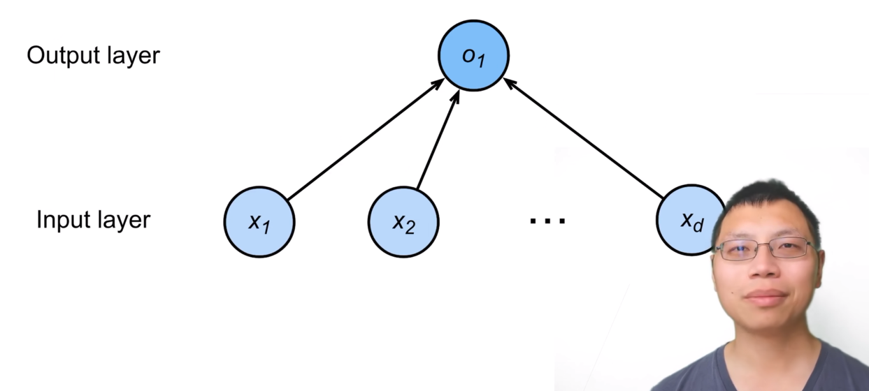
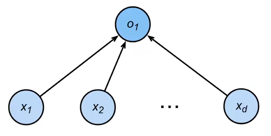
线性模型可以看做是单层神经网络
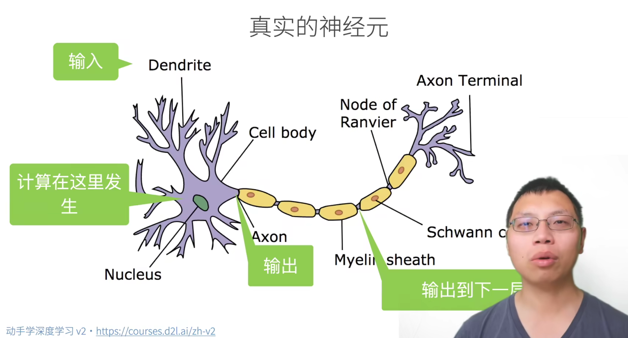
神经网络源于神经科学
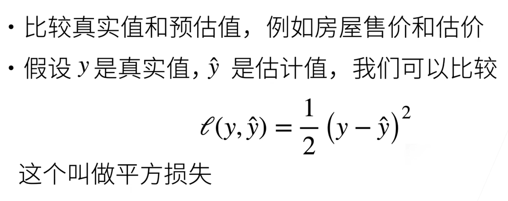
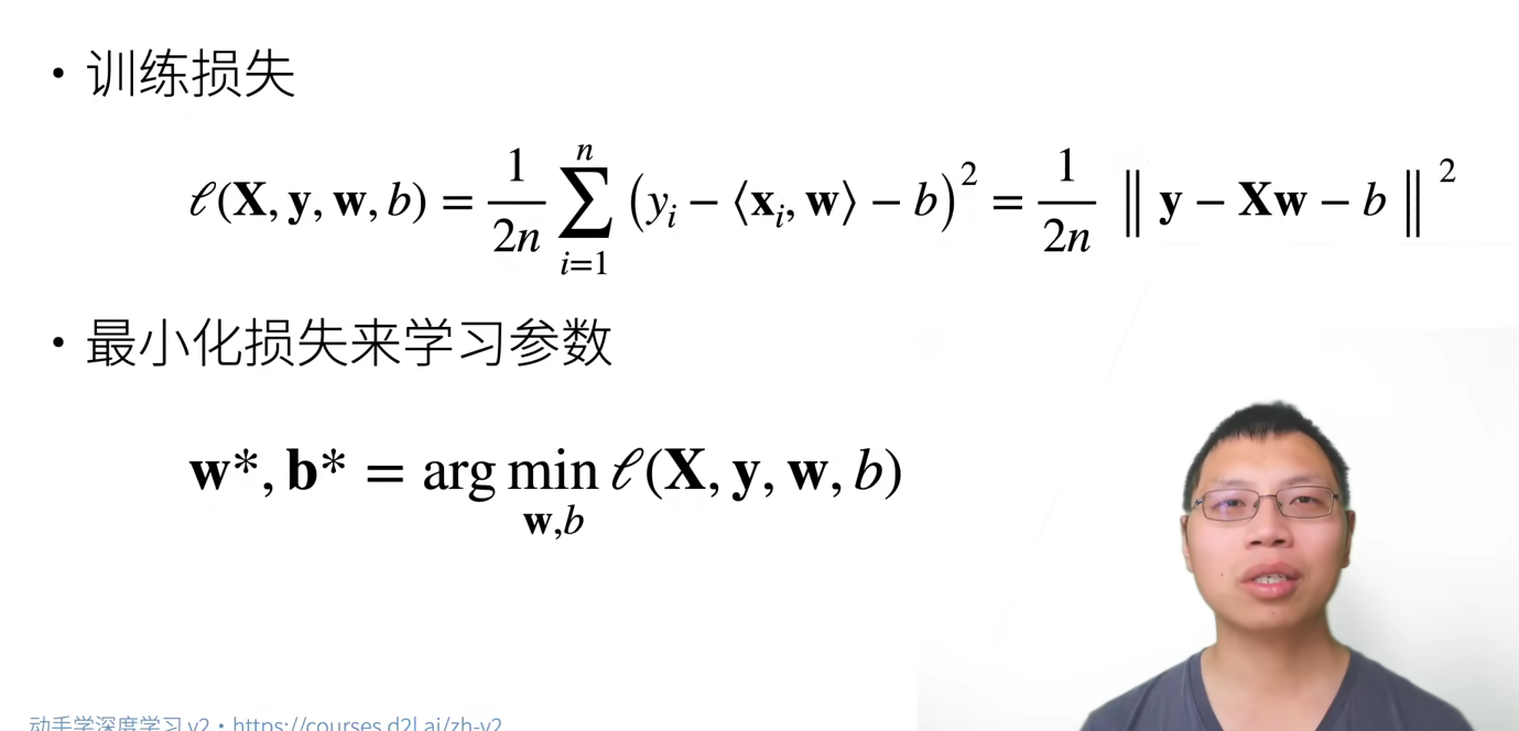
衡量预估质量
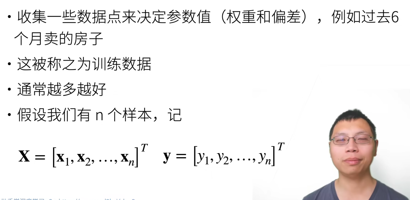
训练数据
参数学习
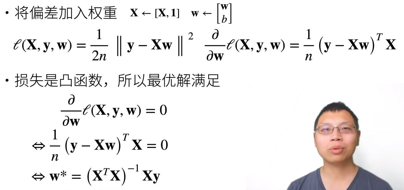
显示解
总结 基础优化方法
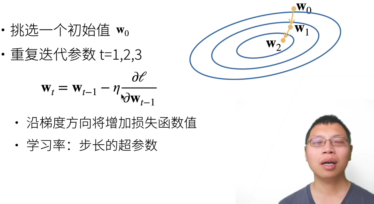
梯度下降
选择学习率
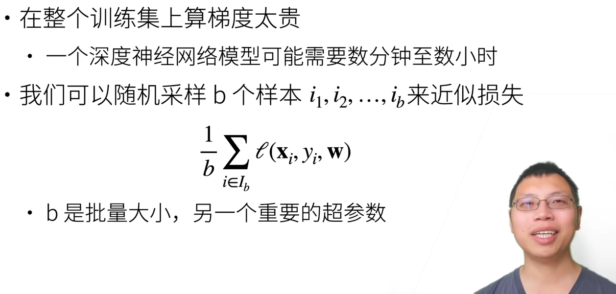
小批量随机梯度下降
选择批量大小
总结
线性回归的从零开始实现 我们将从零开始实现整个方法,包括数据流水线、模型、损失函数和小批量随机梯度下降优化器
1 2 3 4 5 6 7 %matplotlib inline import math import time import numpy as np import torch from d2l import torch as d2l
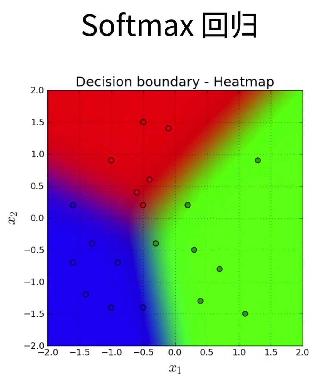
09 Softmax 回归 + 损失函数 + 图片分类数据集
回归 vs 分类
回归估计一个连续值
分类预测一个离散类别
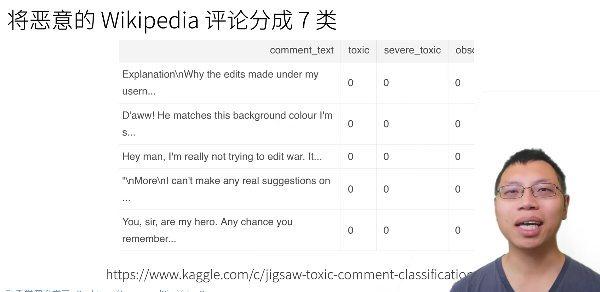
Kaggle上的分类问题
从回归到多类分类 回归
单连续数值输出
自然区间R
跟真实值的区别作为损失分类
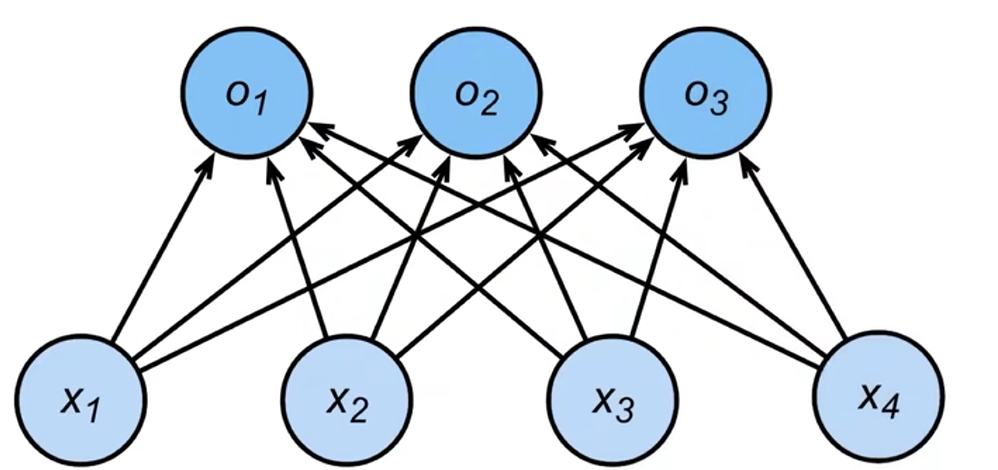
通常多个输出
输出i是预测为第i类的置信度
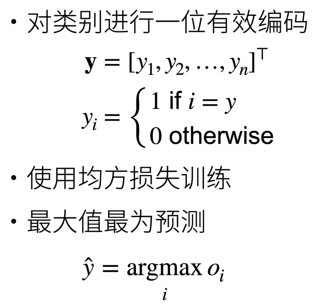
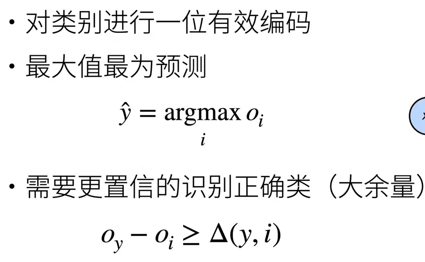
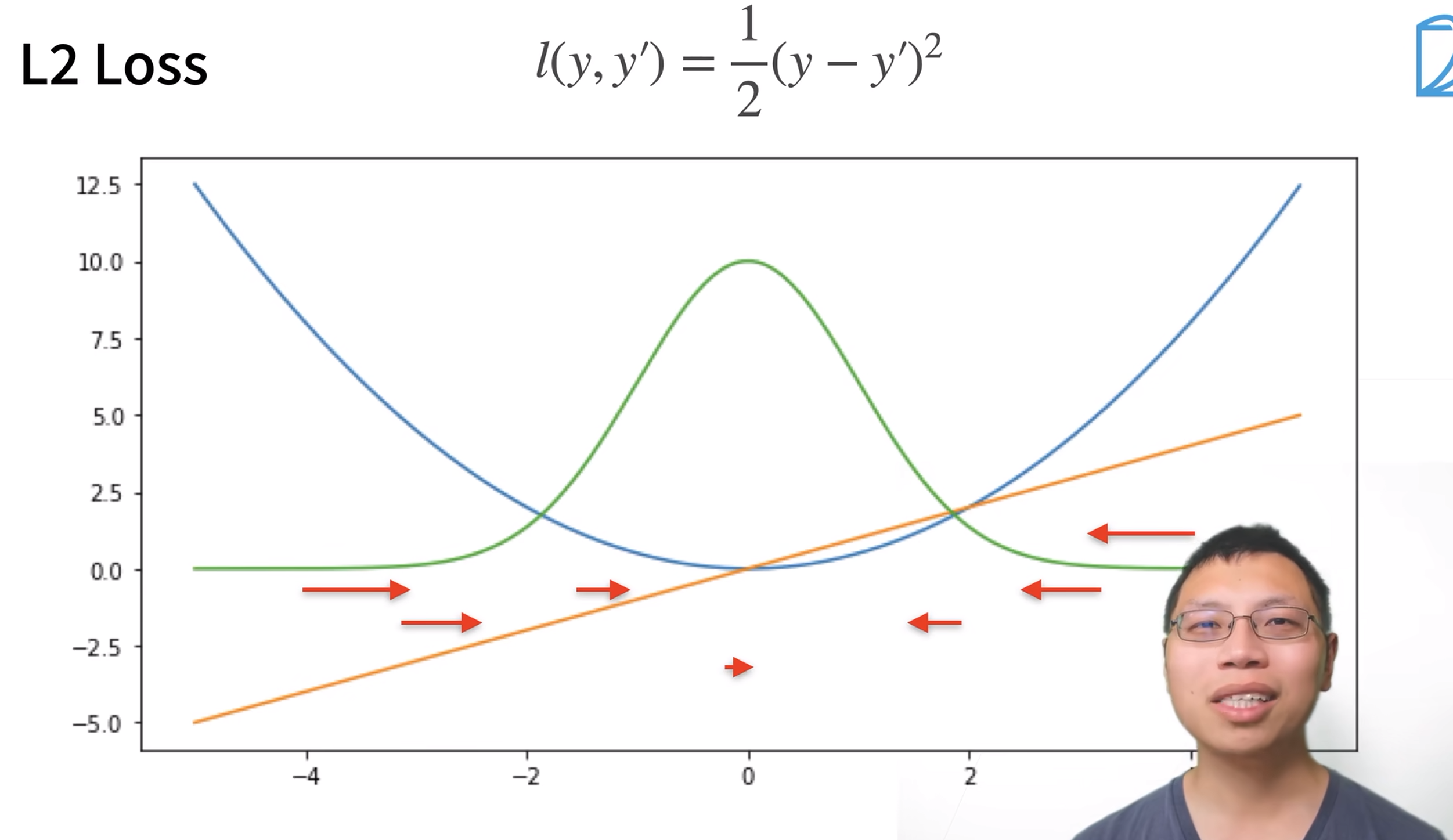
从回归到多类分类——均方损失
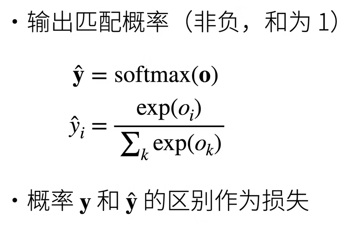
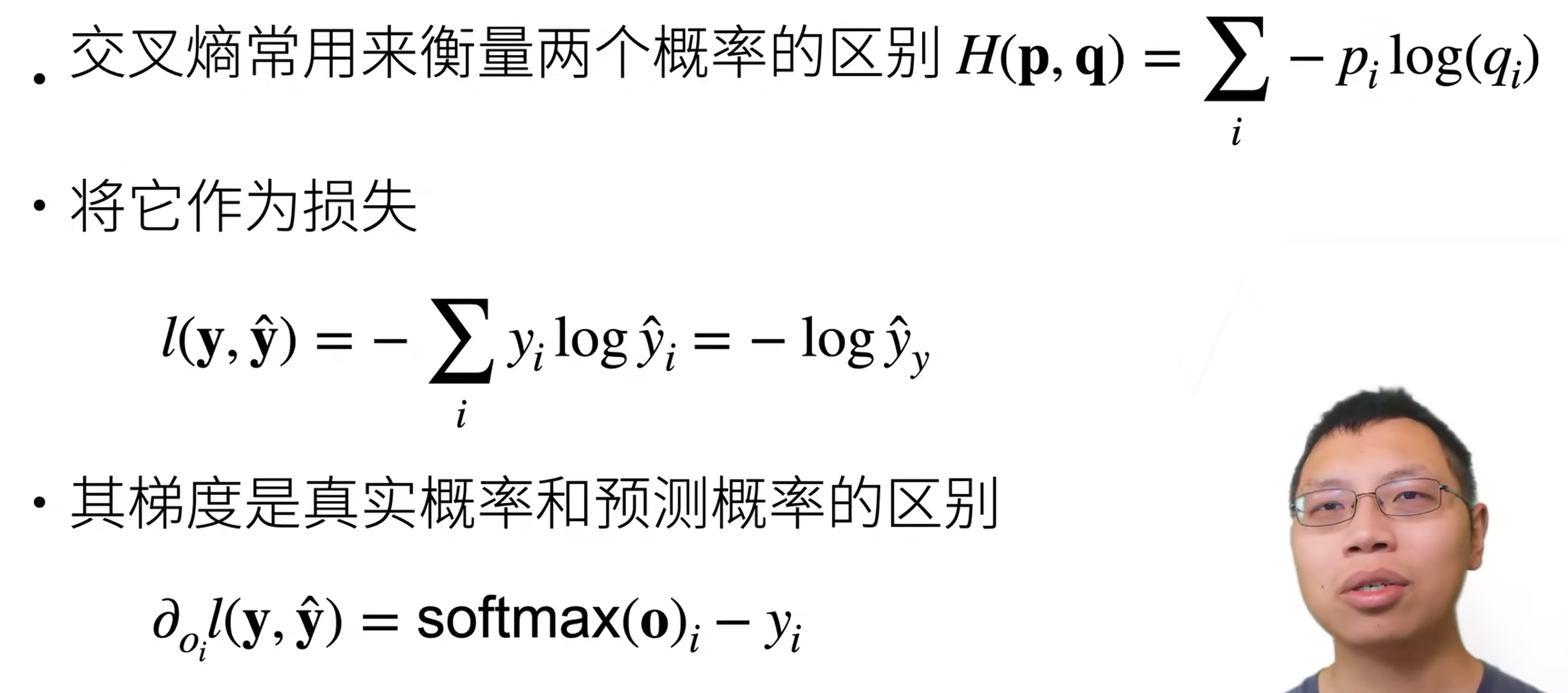
Softmax和交叉熵损失
总结
Softmax回归是一个多类分类模型
使用Softmax操作得到每个类的预测置信度
使用交叉熵来衡量预测和标号的区别
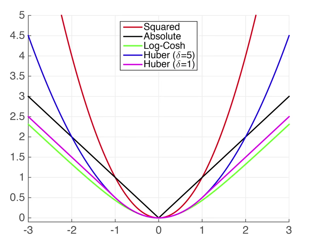
损失函数 用来衡量预测值和真实值之间的区别
均方损失函数
绝对值损失函数
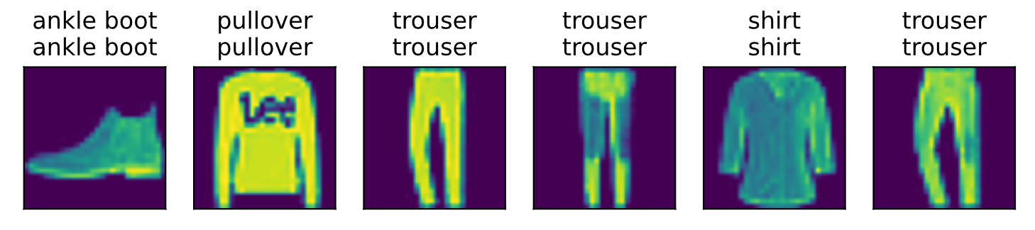
softmax回归的从零开始实现 就像我们从零开始实现线性回归一样, 你应该知道实现softmax的细节
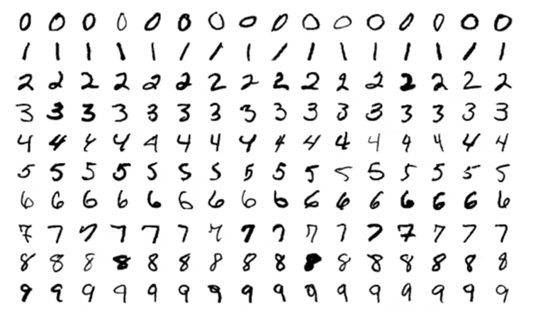
1 2 3 4 5 6 7 import torch from IPython import display from d2l import torch as d2l batch_size = 256 #每次随机读取256张图片 train_iter, test_iter = d2l.load_data_fashion_mnist(batch_size) #返回训练集和测试集的迭代器
将展平每个图像,把它们看作长度为784的向量。 因为我们的数据集有10个类别,所以网络输出维度为 10
1 2 3 4 5 6 7 8 #图片的长和宽都为28,28*28=784 #对于softmax函数而言,输入必须是一个向量,需要把整个图片拉长,拉成一个向量 num_inputs = 784 num_outputs = 10 #定义权重w,初始成一个高斯随机分布的值,均值为0,方差为0.01,形状是行数等于输入的个数、列数等于输出的个数,计算梯度requires_grad=True W = torch.normal(0, 0.01, size=(num_inputs, num_outputs), requires_grad=True) b = torch.zeros(num_outputs, requires_grad=True) #对于每一个输出都需要一个偏移
给定一个矩阵X,我们可以对所有元素求和
1 2 3 4 #定义一个2*3的矩阵 X = torch.tensor([[1.0, 2.0, 3.0], [4.0, 5.0, 6.0]]) #如果按照维度=0来求和的话 X.sum(0, keepdim=True), X.sum(1, keepdim=True)
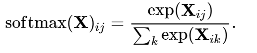
实现softmax
1 2 3 4 def softmax(X): X_exp = torch.exp(X) #对每个元素做指数计算 partition = X_exp.sum(1, keepdim=True) #按照维度为1来求和 return X_exp / partition #广播机制:X_exp的每一行除以partition对应行的那个数
我们将每个元素变成一个非负数。此外,依据概率原理,每行总和为1
1 2 3 X = torch.normal(0, 1, (2, 5)) #创建一个随机的均值为0,方差为1的两行五列的矩阵X X_prob = softmax(X) #将X放入softmax函数 X_prob, X_prob.sum(1)
实现softmax回归模型
1 2 def net(X): return softmax(torch.matmul(X.reshape((-1, W.shape[0])), W) + b)
创建一个数据y_hat,其中包含2个样本在3个类别的预测概率, 使用y作为y_hat中概率的索引
1 2 3 y = torch.tensor([0, 2]) y_hat = torch.tensor([[0.1, 0.3, 0.6], [0.3, 0.2, 0.5]]) y_hat[[0, 1], y]
10多层感知机
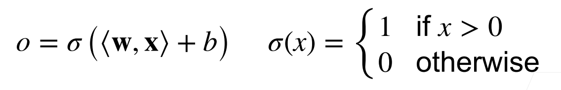
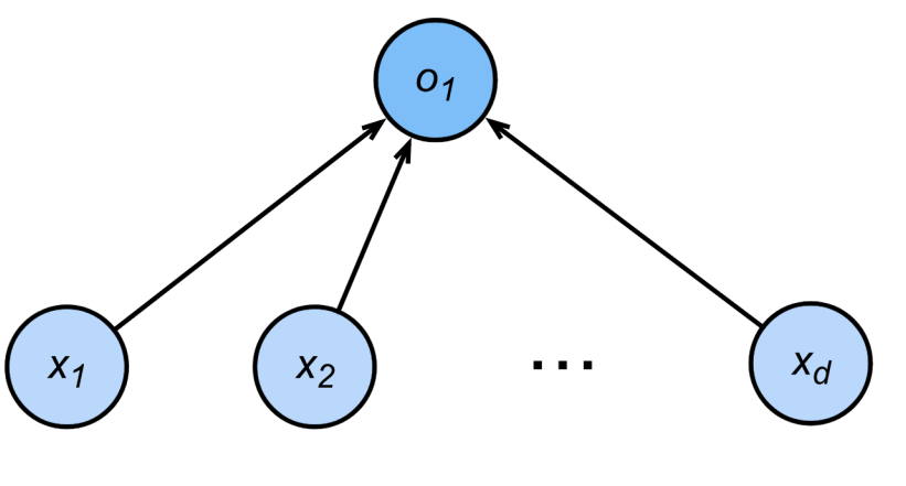
感知机
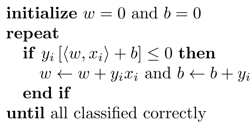
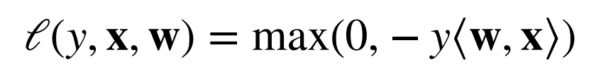
训练感知机 预测和真实值如果准确就是同号,预测错误就是异号
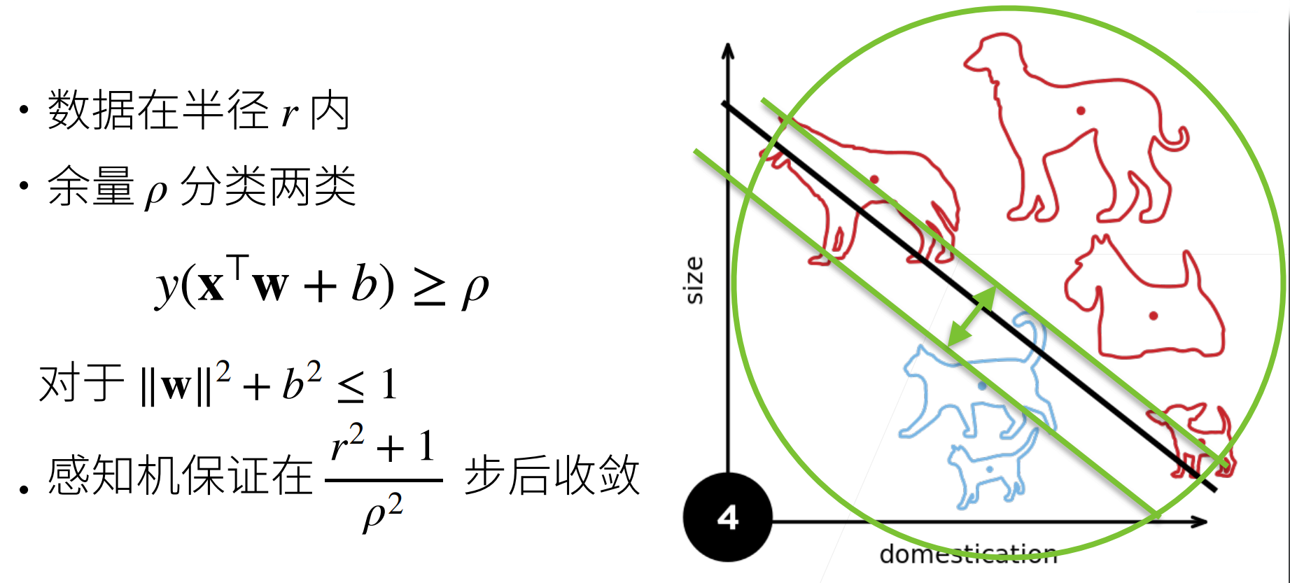
收敛定理
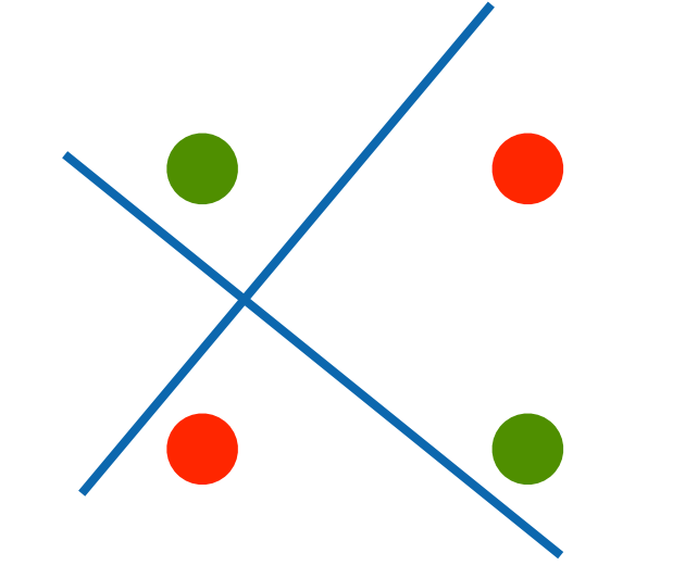
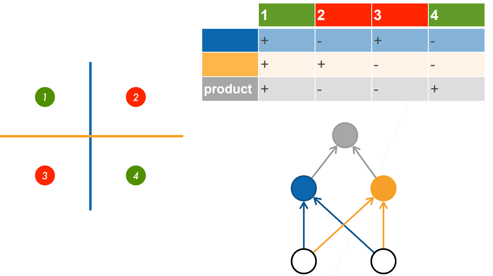
XOR问题(Minsky & Papert,1969) 感知机不能拟合XOR函数,它智能产生线性分割面
总结
感知机是一个二分类模型,是最早的AI模型之一
它的求解算法等价于使用批量大小为1的梯度下降
它不能拟合XOR函数,导致的第一次AI寒冬
多层感知机
学习XOR
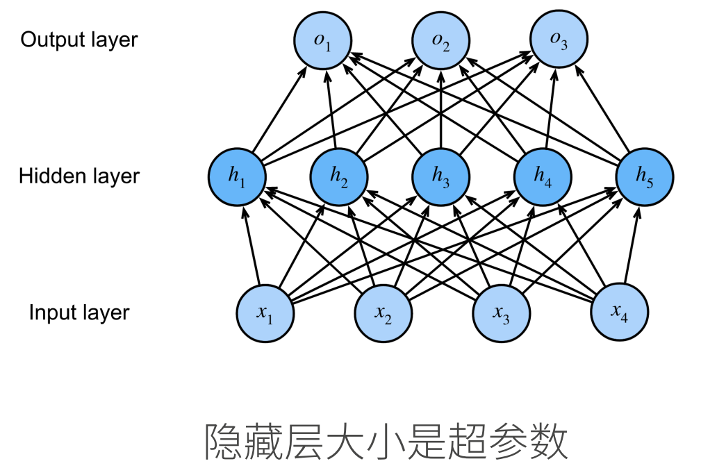
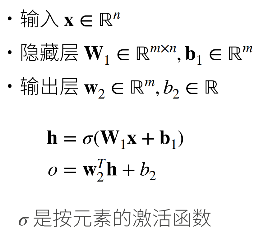
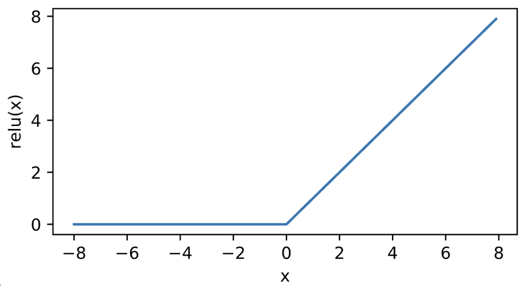
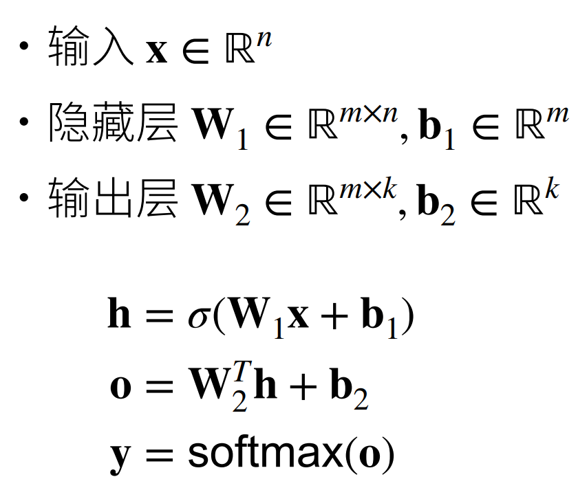
单隐藏层
单隐藏层——单分类
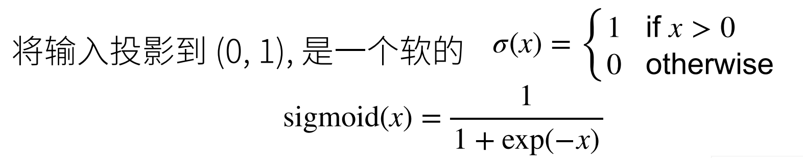
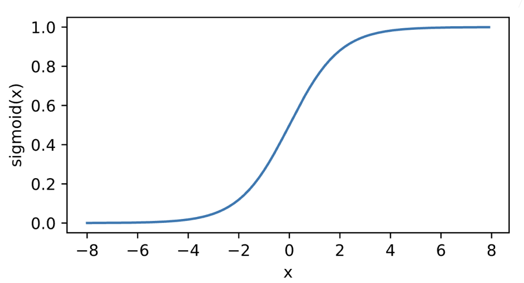
Sigmoid激活函数
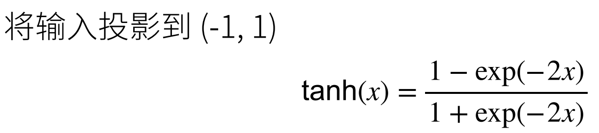
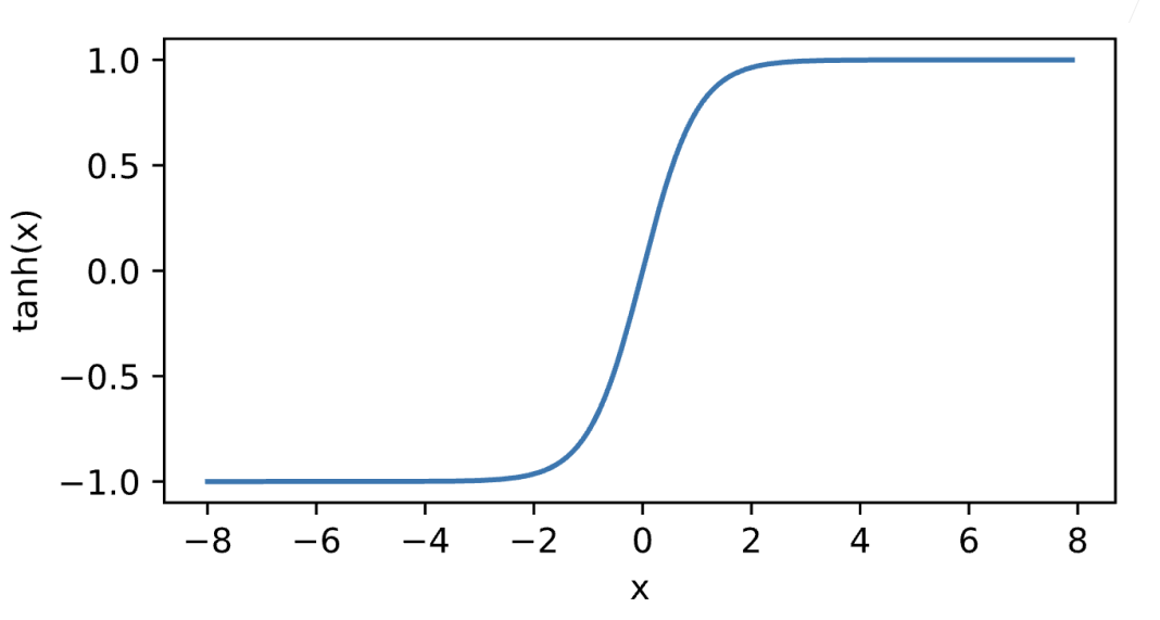
Tanh激活函数
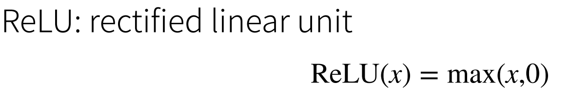
ReLU激活函数
多类分类
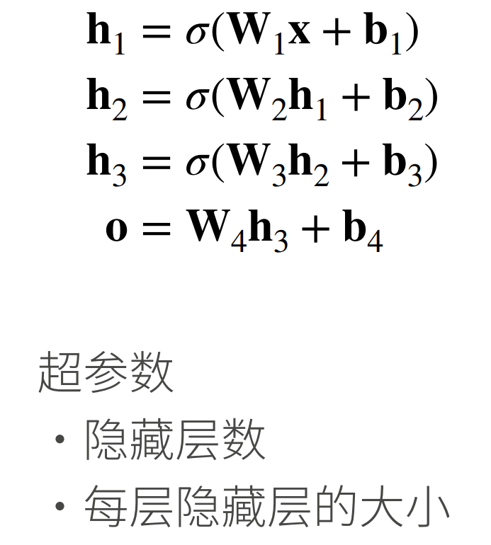
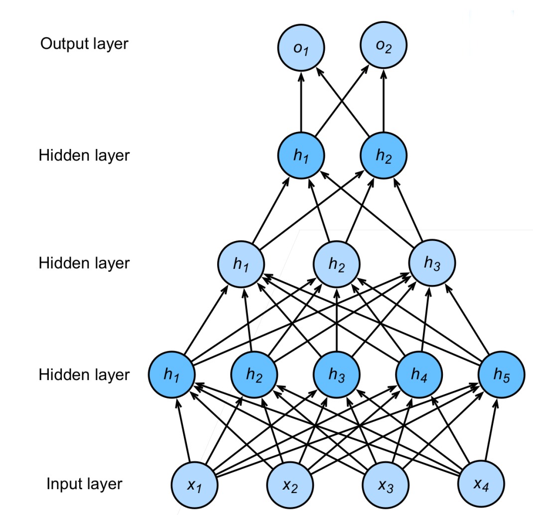
多隐藏层
总结
多层感知机使用隐藏层和激活函数来得到非线性模型
常用激活函数是Sigmoid,Tanh,ReLU
使用Softmax来处理多类分类
超参数为隐藏层数,和各个隐藏层大小
代码 多层感知机的从零开始实现
1 2 3 4 5 6 import torch from torch import nn from d2l import torch as d2l batch_size = 256 train_iter, test_iter = d2l.load_data_fashion_mnist(batch_size)
实现一个具有单隐藏层的多层感知机,它包含256个隐藏单元
1 2 3 4 5 6 7 8 9 10 num_inputs, num_outputs, num_hiddens = 784, 10, 256 W1 = nn.Parameter( torch.randn(num_inputs, num_hiddens, requires_grad=True) * 0.01) b1 = nn.Parameter(torch.zeros(num_hiddens, requires_grad=True)) W2 = nn.Parameter( torch.randn(num_hiddens, num_outputs, requires_grad=True) * 0.01) b2 = nn.Parameter(torch.zeros(num_outputs, requires_grad=True)) params = [W1, b1, W2, b2]
实现ReLU激活函数
1 2 3 def relu(X): a = torch.zeros_like(X) return torch.max(X, a)
实现我们的模型
1 2 3 4 5 6 def net(X): X = X.reshape((-1, num_inputs)) H = relu(X @ W1 + b1) return (H @ W2 + b2) loss = nn.CrossEntropyLoss()
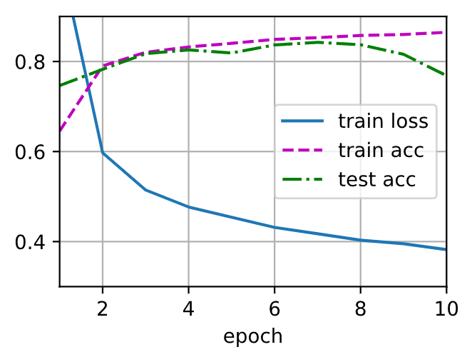
多层感知机的训练过程与softmax回归的训练过程完全相同
1 2 3 num_epochs, lr = 10, 0.1 updater = torch.optim.SGD(params, lr=lr) d2l.train_ch3(net, train_iter, test_iter, loss, num_epochs, updater)
在一些测试数据上应用这个模型
1 d2l.predict_ch3(net, test_iter)
11模型选择 + 过拟合和欠拟合 训练误差和泛化误差
训练误差:模型在训练数据上的误差
泛化误差:模型在新数据上的误差
例子:根据摸考成绩来预测未来考试分数
在过去的考试中表现很好(训练误差)不代表未来考试一定会好(泛化误差)
学生A通过背书在摸考中拿到很好成绩
学生B知道答案后面的原因
验证数据集和测试数据集
验证数据集:一个用来评估模型好坏的数据集
例如拿出50%的训练数据
不要跟训练数据混在一起(常犯错误)
测试数据集:只用一次的数据集。例如
未来的考试
我出价的房子的实际成交价
用在Kaggle私有排行榜中的数据集
K-则交叉验证
在没有足够多数据时使用((这是常态)
算法:
将训练数据分割成K块-
For i= 1,…,K
报告K个验证集误差的平均
常用:K=5或10
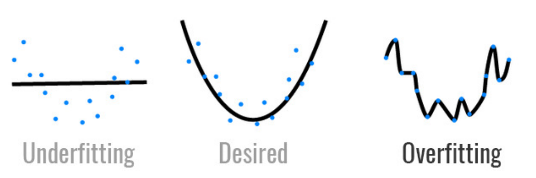
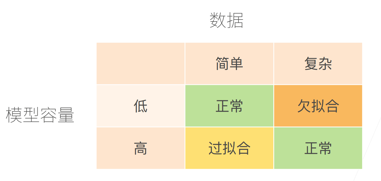
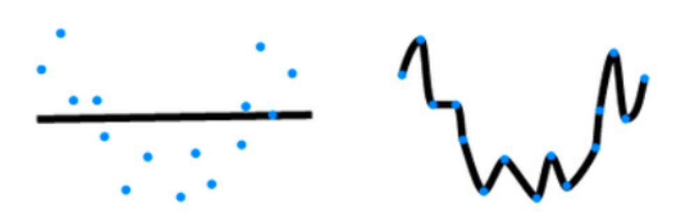
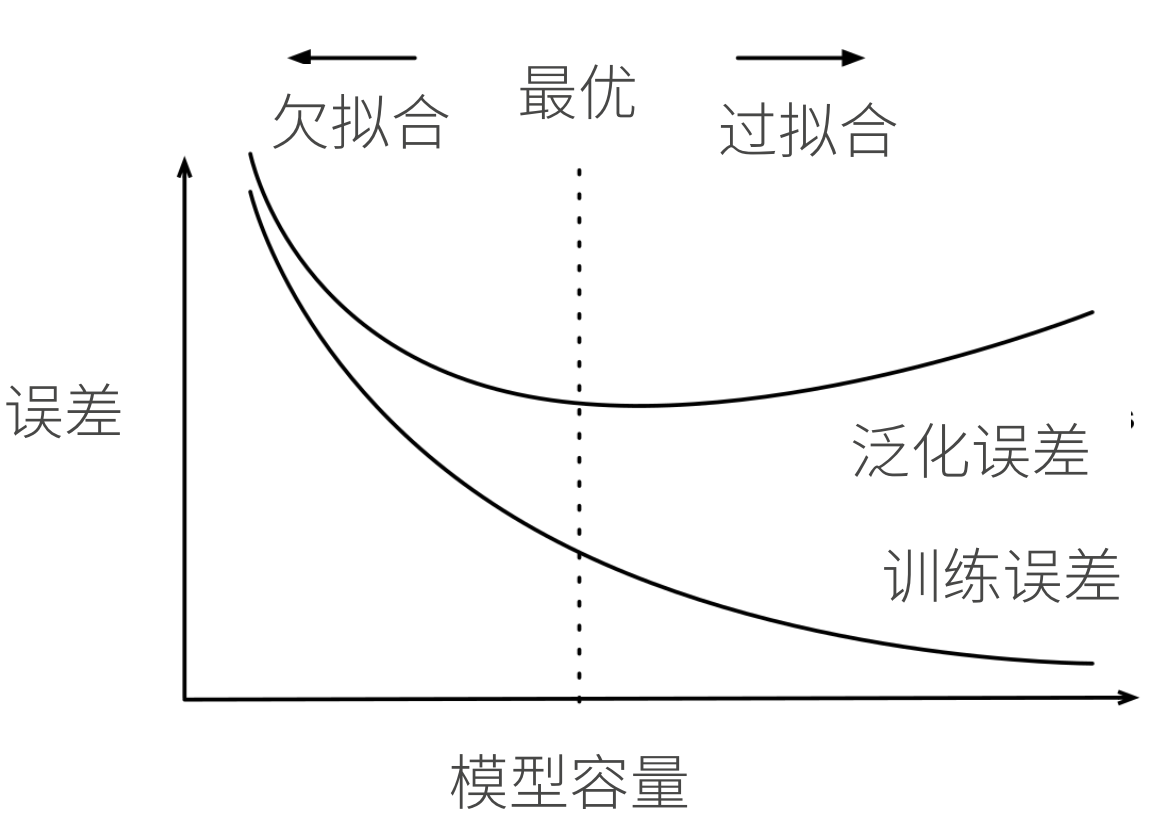
过拟合和欠拟合
模型容量
拟合各种函数的能力
低容量的模型难以拟合训练数据
高容量的模型可以记住所有的训练数据
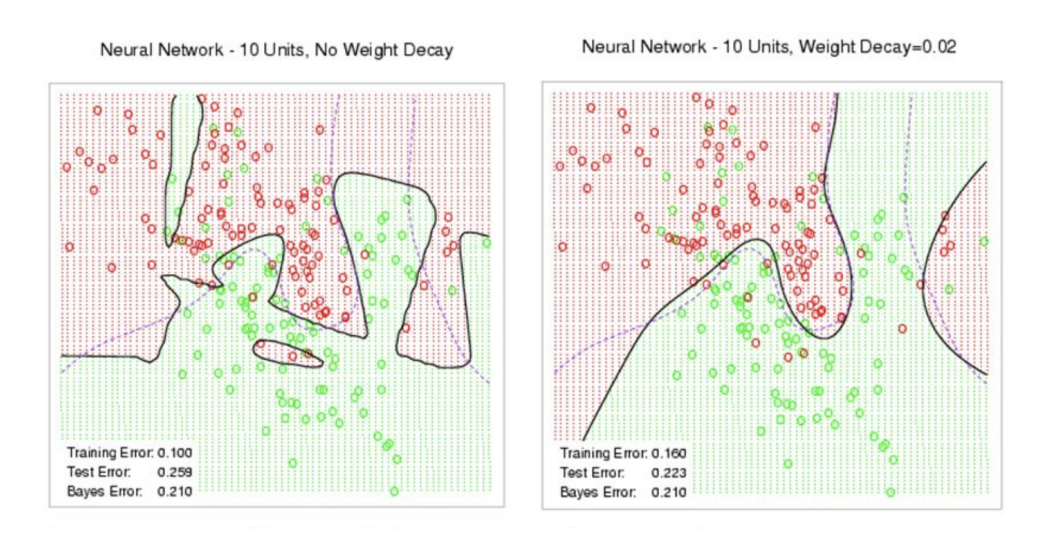
模型容量的影响
估计模型容量
难以在不同的种类算法之间比较
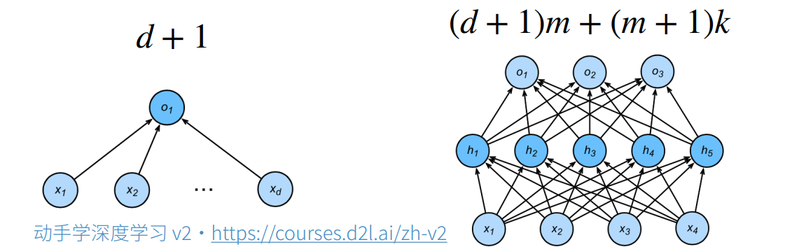
给定一个模型种类,将有两个主要因素
参数的个数
参数值的选择范围
VC维
统计学习理论的一个核心思想
对于一个分类模型,VC等于一个最大的数据集的大小,不管如何给定标号,都存在一个模型来对它进行完美分类
线性分类器的VC维
支持N维输入的感知机的VC维是N+1
—些多层感知机的VC维O(N $log_2$ N)
VC维的用处
提供为什么一个模型好的理论依据
但深度学习中很少使用
数据复杂度
总结
模型容量需要匹配数据复杂度,否则可能导致欠拟合和过拟合
统计机器学习提供数学工具来衡量模型复杂度
实际中一般靠观察训练误差和验证误差
代码 模型选择、欠拟合和过拟合
1 2 3 4 5 import math import numpy as np import torch from torch import nn from d2l import torch as d2l
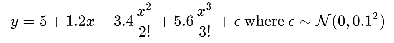
使用以下三阶多项式来生成训练和测试数据的标签:
1 2 3 4 5 6 7 8 9 10 11 12 max_degree = 20 n_train, n_test = 100, 100 true_w = np.zeros(max_degree) true_w[0:4] = np.array([5, 1.2, -3.4, 5.6]) features = np.random.normal(size=(n_train + n_test, 1)) np.random.shuffle(features) poly_features = np.power(features, np.arange(max_degree).reshape(1, -1)) for i in range(max_degree): poly_features[:, i] /= math.gamma(i + 1) labels = np.dot(poly_features, true_w) labels += np.random.normal(scale=0.1, size=labels.shape)
看一下前2个样本
1 2 3 4 5 true_w, features, poly_features, labels = [ torch.tensor(x, dtype=torch.float32) for x in [true_w, features, poly_features, labels]] features[:2], poly_features[:2, :], labels[:2]
实现一个函数来评估模型在给定数据集上的损失
1 2 3 4 5 6 7 8 9 def evaluate_loss(net, data_iter, loss): """评估给定数据集上模型的损失。""" metric = d2l.Accumulator(2) for X, y in data_iter: out = net(X) y = y.reshape(out.shape) l = loss(out, y) metric.add(l.sum(), l.numel()) return metric[0] / metric[1]
定义训练函数
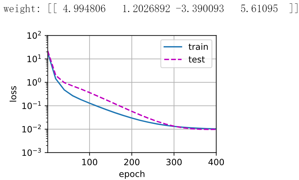
1 2 3 4 5 6 7 8 9 10 11 12 13 14 15 16 17 18 19 20 def train(train_features, test_features, train_labels, test_labels, num_epochs=400): loss = nn.MSELoss() input_shape = train_features.shape[-1] net = nn.Sequential(nn.Linear(input_shape, 1, bias=False)) batch_size = min(10, train_labels.shape[0]) train_iter = d2l.load_array((train_features, train_labels.reshape(-1, 1)), batch_size) test_iter = d2l.load_array((test_features, test_labels.reshape(-1, 1)), batch_size, is_train=False) trainer = torch.optim.SGD(net.parameters(), lr=0.01) animator = d2l.Animator(xlabel='epoch', ylabel='loss', yscale='log', xlim=[1, num_epochs], ylim=[1e-3, 1e2], legend=['train', 'test']) for epoch in range(num_epochs): d2l.train_epoch_ch3(net, train_iter, loss, trainer) if epoch == 0 or (epoch + 1) % 20 == 0: animator.add(epoch + 1, (evaluate_loss( net, train_iter, loss), evaluate_loss(net, test_iter, loss))) print('weight:', net[0].weight.data.numpy())
三阶多项式函数拟合(正态)
1 2 train(poly_features[:n_train, :4], poly_features[n_train:, :4], labels[:n_train], labels[n_train:])
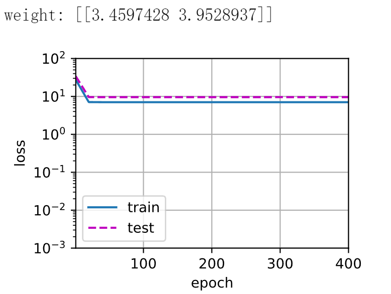
1 2 train(poly_features[:n_train, :2], poly_features[n_train:, :2], labels[:n_train], labels[n_train:])
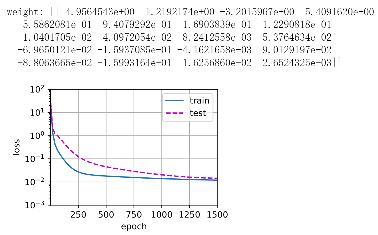
1 2 train(poly_features[:n_train, :], poly_features[n_train:, :], labels[:n_train], labels[n_train:], num_epochs=1500)
12权重衰退
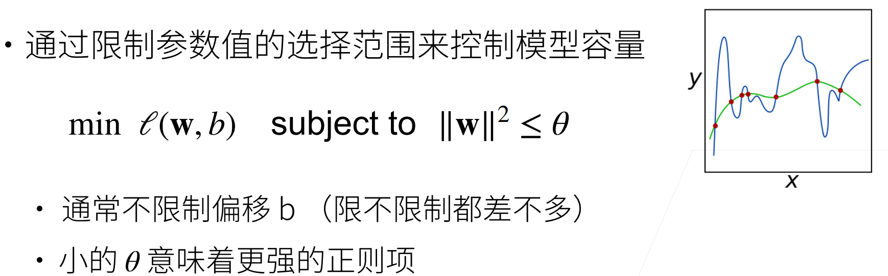
使用均方范数作为硬性限制
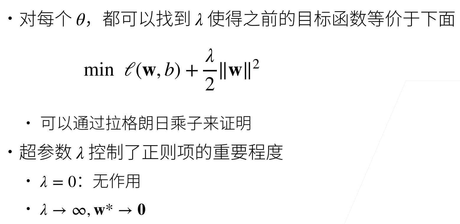
使用均方范数作为柔性限制
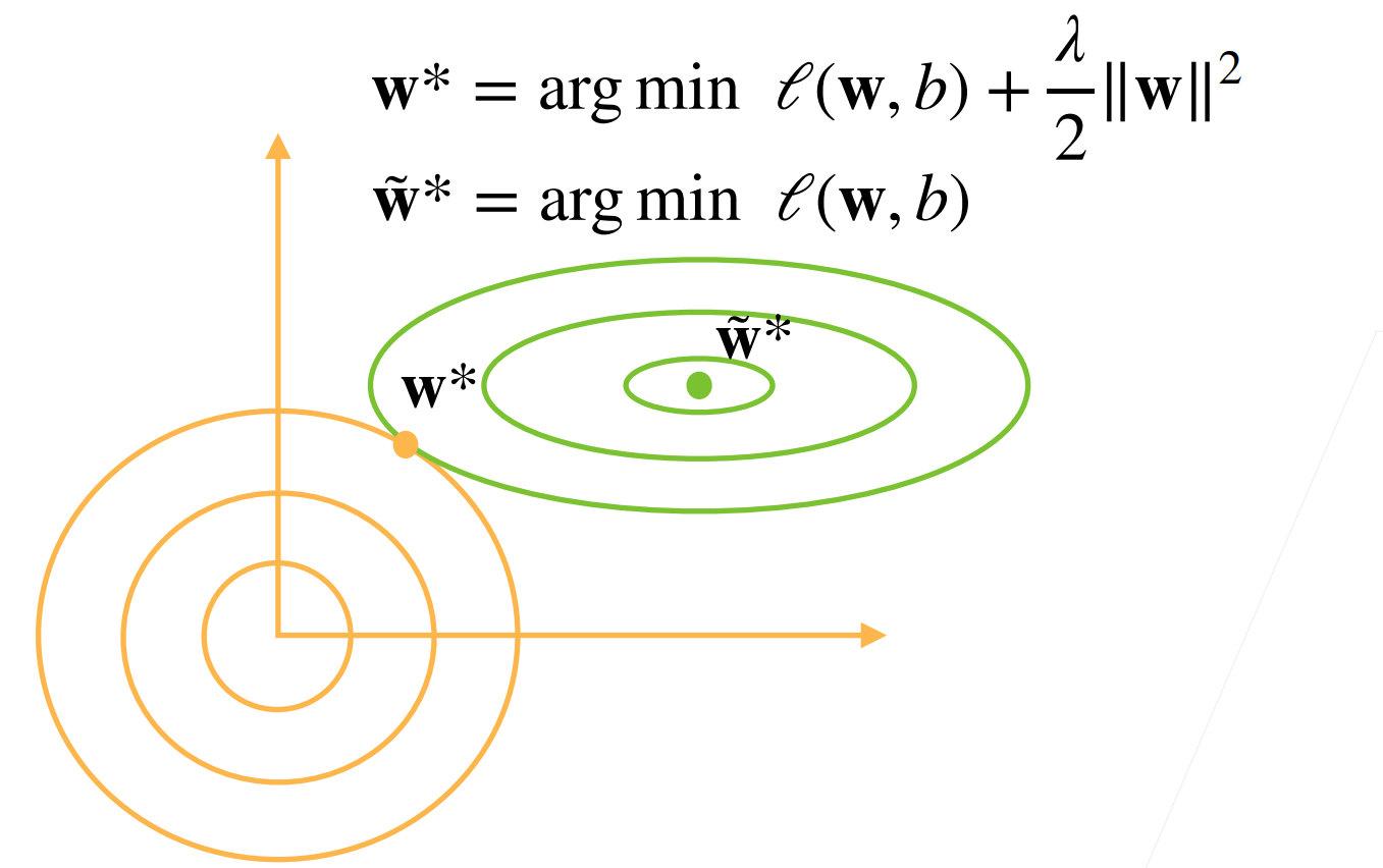
演示对最优解的影响
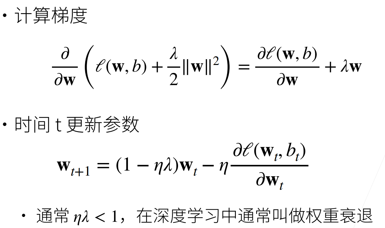
参数更新法则
总结
权重衰退通过L2正则项使得模型参数不会过大,从而控制模型复杂度
正则项权重是控制模型复杂度的超参数
代码 权重衰减是最广泛使用的正则化的技术之一
1 2 3 4 %matplotlib inline import torch from torch import nn from d2l import torch as d2l
像以前一样生成一些数据
1 2 3 4 5 6 n_train, n_test, num_inputs, batch_size = 20, 100, 200, 5 true_w, true_b = torch.ones((num_inputs, 1)) * 0.01, 0.05 train_data = d2l.synthetic_data(true_w, true_b, n_train) train_iter = d2l.load_array(train_data, batch_size) test_data = d2l.synthetic_data(true_w, true_b, n_test) test_iter = d2l.load_array(test_data, batch_size, is_train=False)
初始化模型参数
1 2 3 4 def init_params(): w = torch.normal(0, 1, size=(num_inputs, 1), requires_grad=True) b = torch.zeros(1, requires_grad=True) return [w, b]
定义L2范数惩罚
1 2 def l2_penalty(w): return torch.sum(w.pow(2)) / 2
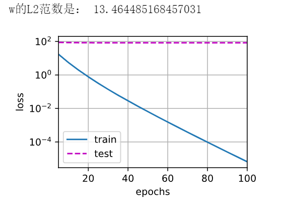
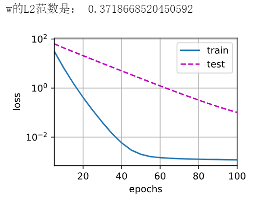
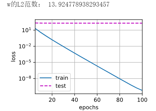
定义训练代码实现
1 2 3 4 5 6 7 8 9 10 11 12 13 14 15 16 def train(lambd): w, b = init_params() net, loss = lambda X: d2l.linreg(X, w, b), d2l.squared_loss num_epochs, lr = 100, 0.003 animator = d2l.Animator(xlabel='epochs', ylabel='loss', yscale='log', xlim=[5, num_epochs], legend=['train', 'test']) for epoch in range(num_epochs): for X, y in train_iter: with torch.enable_grad(): l = loss(net(X), y) + lambd * l2_penalty(w) l.sum().backward() d2l.sgd([w, b], lr, batch_size) if (epoch + 1) % 5 == 0: animator.add(epoch + 1, (d2l.evaluate_loss(net, train_iter, loss), d2l.evaluate_loss(net, test_iter, loss))) print('w的L2范数是:', torch.norm(w).item())
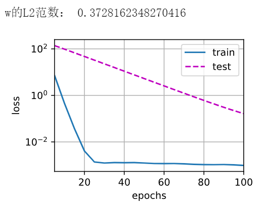
忽略正则化直接训练
1 2 3 4 5 6 7 8 9 10 11 12 13 14 15 16 17 18 19 20 21 22 23 def train_concise(wd): net = nn.Sequential(nn.Linear(num_inputs, 1)) for param in net.parameters(): param.data.normal_() loss = nn.MSELoss() num_epochs, lr = 100, 0.003 trainer = torch.optim.SGD([{ "params": net[0].weight, 'weight_decay': wd}, { "params": net[0].bias}], lr=lr) animator = d2l.Animator(xlabel='epochs', ylabel='loss', yscale='log', xlim=[5, num_epochs], legend=['train', 'test']) for epoch in range(num_epochs): for X, y in train_iter: with torch.enable_grad(): trainer.zero_grad() l = loss(net(X), y) l.backward() trainer.step() if (epoch + 1) % 5 == 0: animator.add(epoch + 1, (d2l.evaluate_loss(net, train_iter, loss), d2l.evaluate_loss(net, test_iter, loss))) print('w的L2范数:', net[0].weight.norm().item())
这些图看起来和我们从零开始实现权重衰减时的图相同
13丢弃法 动机
一个好的模型需要对输入数据的扰动鲁棒
使用有噪音的数据等价于Tikhonov正则
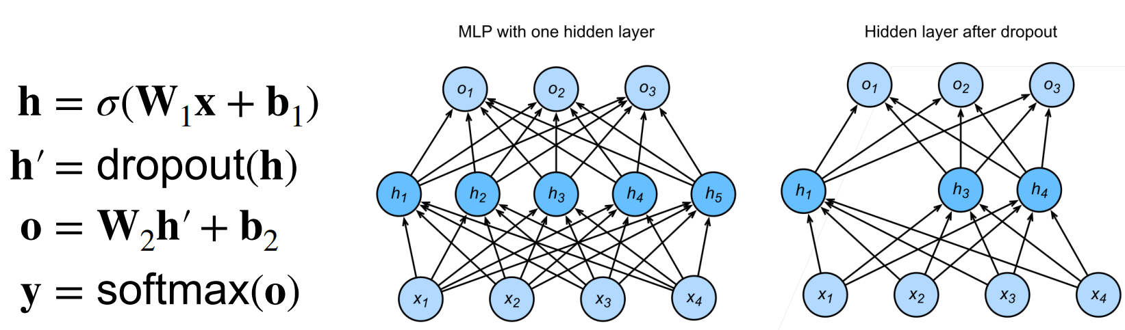
丢弃法:在层之间加入噪音
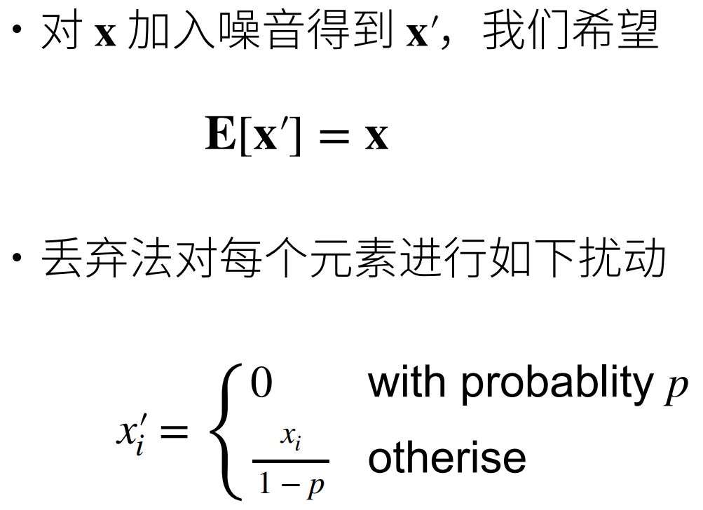
无偏差的加入噪音
使用丢弃法 通常将丢弃法作用在隐藏全连接层的输出上
推理中的丢弃法
正则项只在训练中使用:他们影响模型参数的更新
在推理过程中,丢弃法直接返回输入h = dropout(h)
总结
丢弃法将一些输出项随机置0来控制模型复杂度
常作用在多层感知机的隐藏层输出上
丢弃概率是控制模型复杂度的超参数
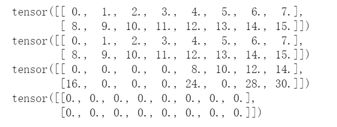
代码 我们实现dropout_layer函数,该函数以dropout的概率丢弃张量输入X中的元素
1 2 3 4 5 6 7 8 9 10 11 12 13 import torch from torch import nn from d2l import torch as d2l def dropout_layer(X, dropout): assert 0 <= dropout <= 1 if dropout == 1: return torch.zeros_like(X) if dropout == 0: return X mask = (torch.Tensor(X.shape).uniform_(0, 1) > dropout).float() return mask * X / (1.0 - dropout)
测试dropout_layer函数
1 2 3 4 5 X = torch.arange(16, dtype=torch.float32).reshape((2, 8)) print(X) print(dropout_layer(X, 0.)) print(dropout_layer(X, 0.5)) print(dropout_layer(X, 1.))
1 2 3 4 5 6 7 8 9 10 11 12 13 14 15 16 17 18 19 20 21 22 23 24 25 26 num_inputs, num_outputs, num_hiddens1, num_hiddens2 = 784, 10, 256, 256 dropout1, dropout2 = 0.2, 0.5 class Net(nn.Module): def __init__(self, num_inputs, num_outputs, num_hiddens1, num_hiddens2, is_training=True): super(Net, self).__init__() self.num_inputs = num_inputs self.training = is_training self.lin1 = nn.Linear(num_inputs, num_hiddens1) self.lin2 = nn.Linear(num_hiddens1, num_hiddens2) self.lin3 = nn.Linear(num_hiddens2, num_outputs) self.relu = nn.ReLU() def forward(self, X): H1 = self.relu(self.lin1(X.reshape((-1, self.num_inputs)))) if self.training == True: H1 = dropout_layer(H1, dropout1) H2 = self.relu(self.lin2(H1)) if self.training == True: H2 = dropout_layer(H2, dropout2) out = self.lin3(H2) return out net = Net(num_inputs, num_outputs, num_hiddens1, num_hiddens2)
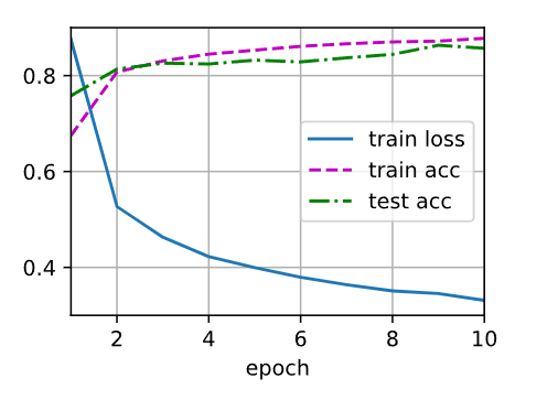
训练和测试
1 2 3 4 5 num_epochs, lr, batch_size = 10, 0.5, 256 loss = nn.CrossEntropyLoss() train_iter, test_iter = d2l.load_data_fashion_mnist(batch_size) trainer = torch.optim.SGD(net.parameters(), lr=lr) d2l.train_ch3(net, train_iter, test_iter, loss, num_epochs, trainer)
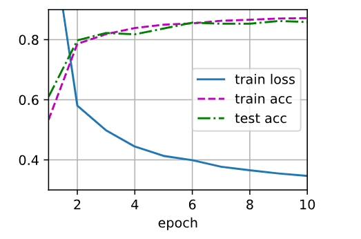
1 2 3 4 5 6 7 8 9 net = nn.Sequential(nn.Flatten(), nn.Linear(784, 256), nn.ReLU(), nn.Dropout(dropout1), nn.Linear(256, 256), nn.ReLU(), nn.Dropout(dropout2), nn.Linear(256, 10)) def init_weights(m): if type(m) == nn.Linear: nn.init.normal_(m.weight, std=0.01) net.apply(init_weights);
对模型进行训练和测试
1 2 trainer = torch.optim.SGD(net.parameters(), lr=lr) d2l.train_ch3(net, train_iter, test_iter, loss, num_epochs, trainer)
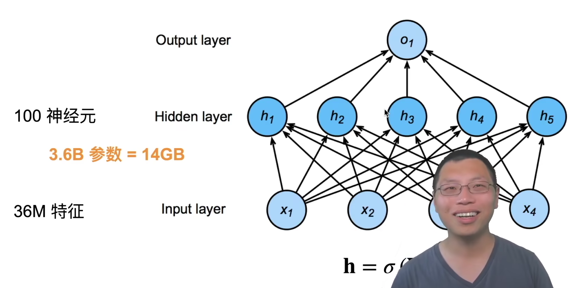
14数值稳定性 + 模型初始化和激活函数 19卷积层 分类猫和狗
使用一个还不错的相机采集图片(12M像素)
RGB图片有36M元素
使用100大小的单隐藏层MLP,模型有3.6B元素
远多于世界上所有猫和狗总算(900M狗,600M猫)
回顾:单隐藏层MLP
两个原则
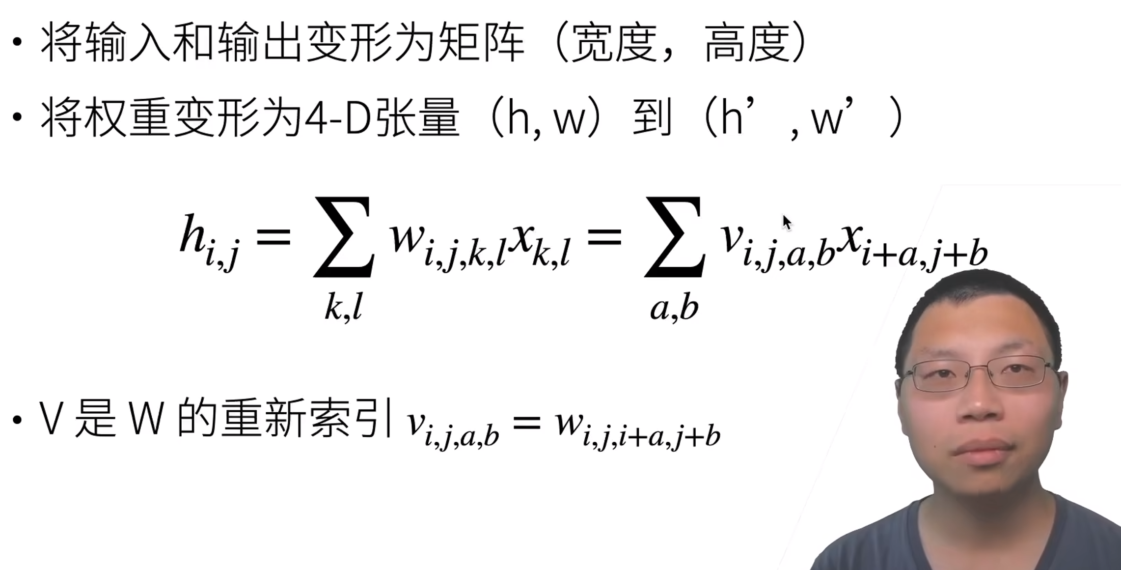
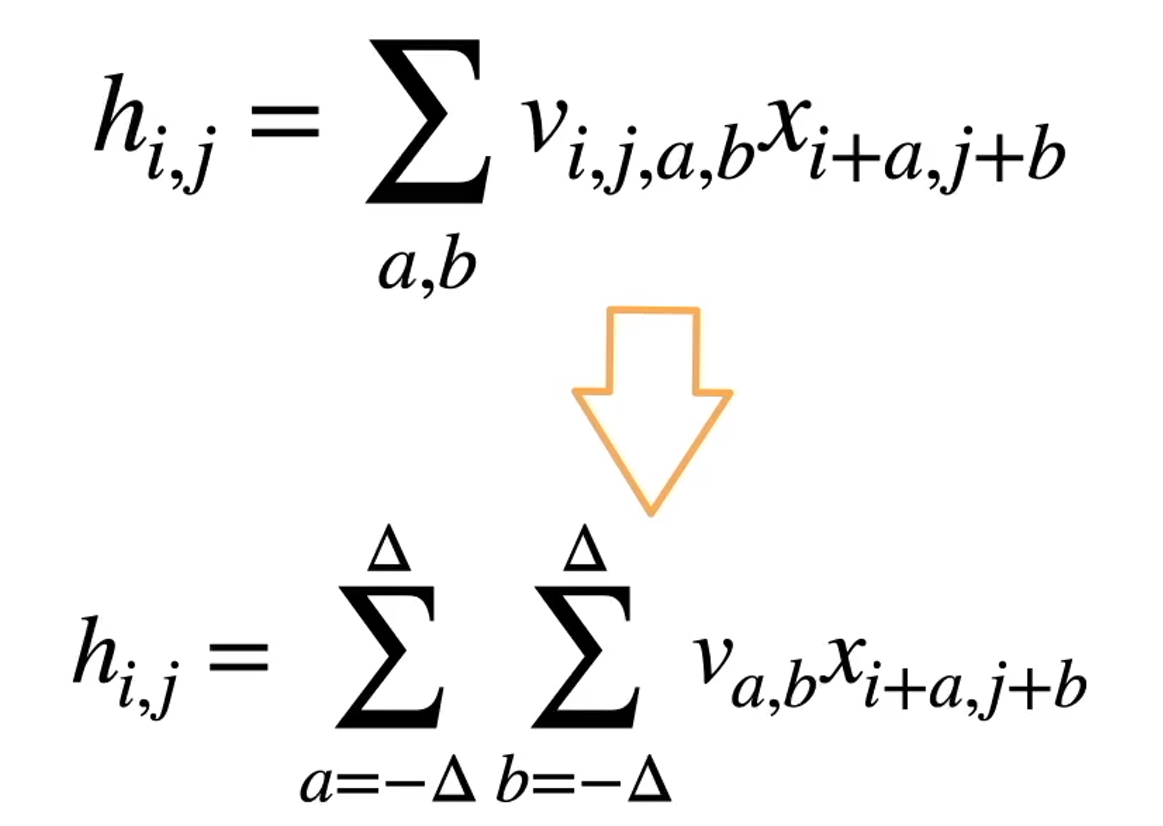
重新考察全连接层
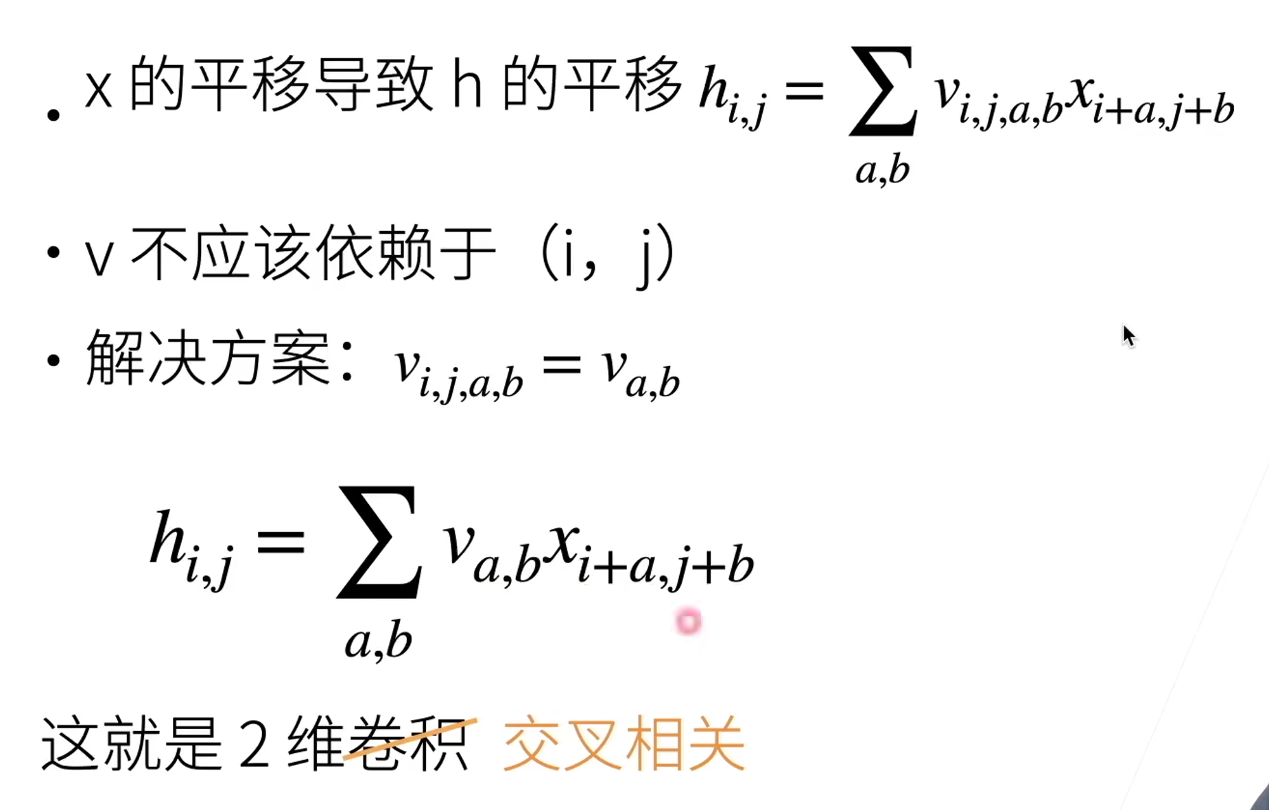
原则1—平移不变性
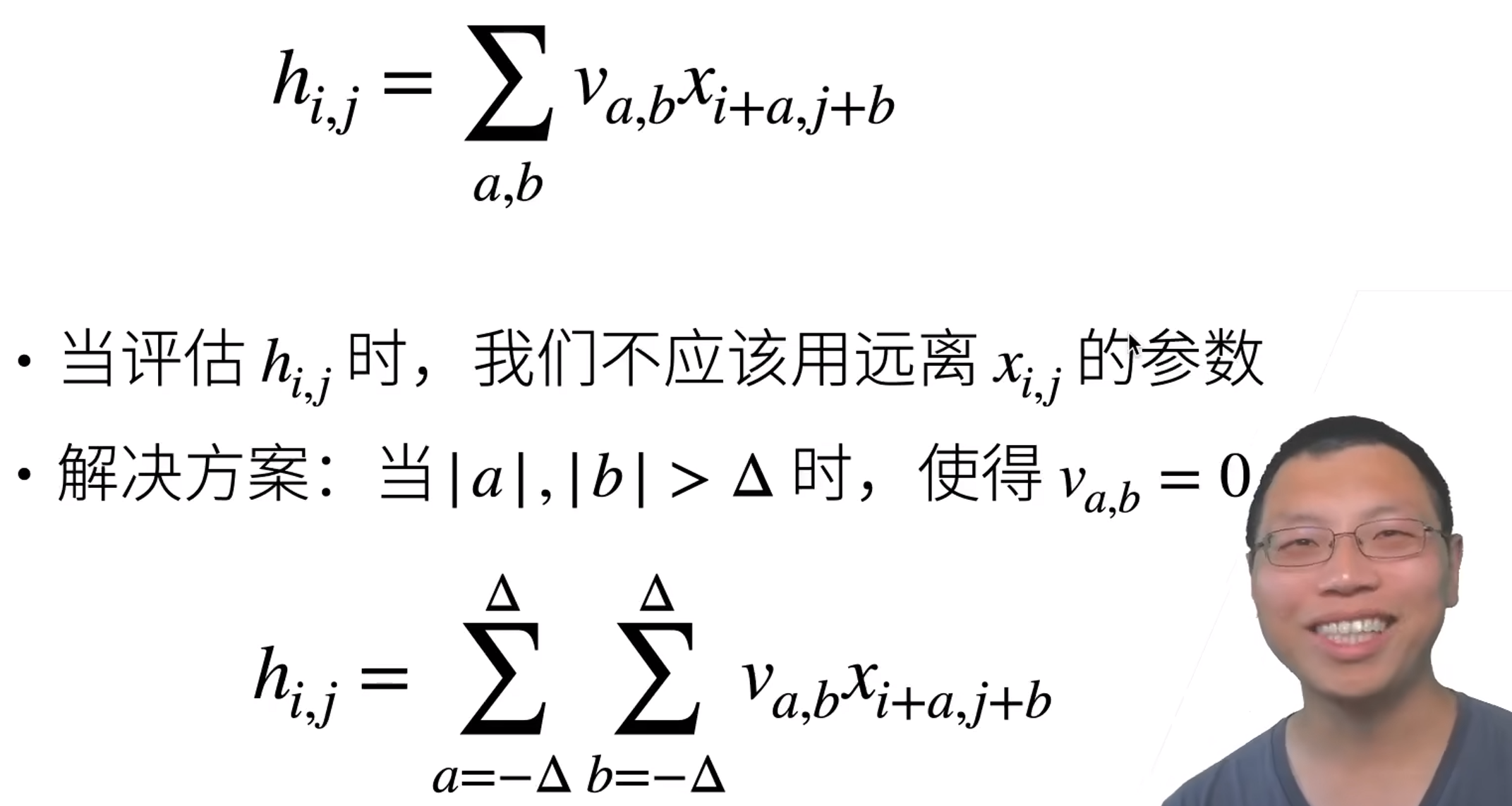
原则2—局部性5 总结
卷积层
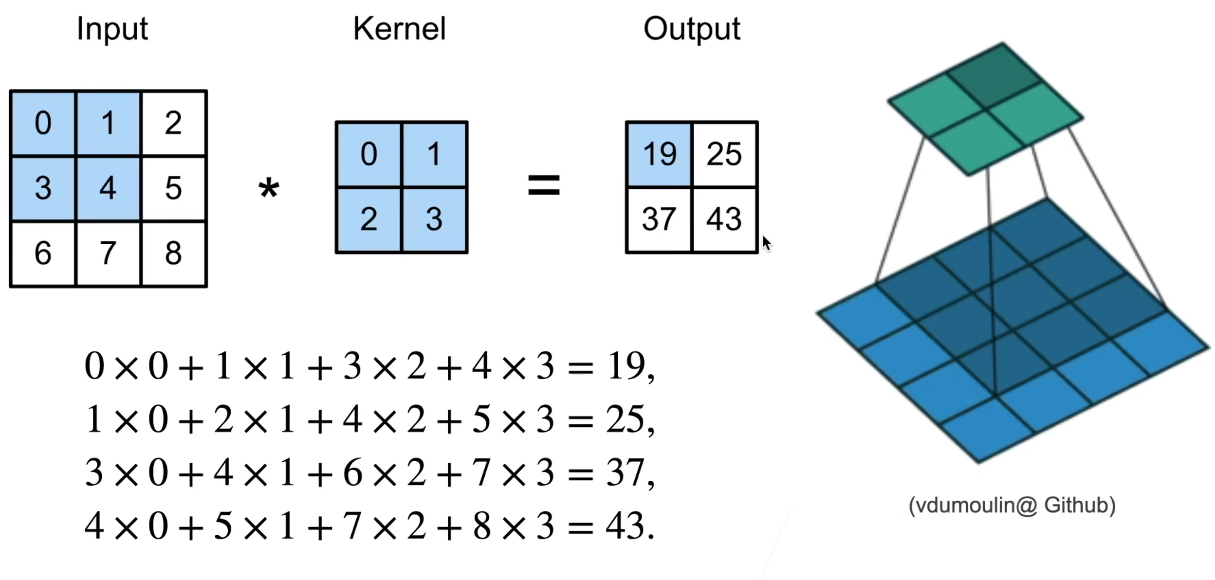
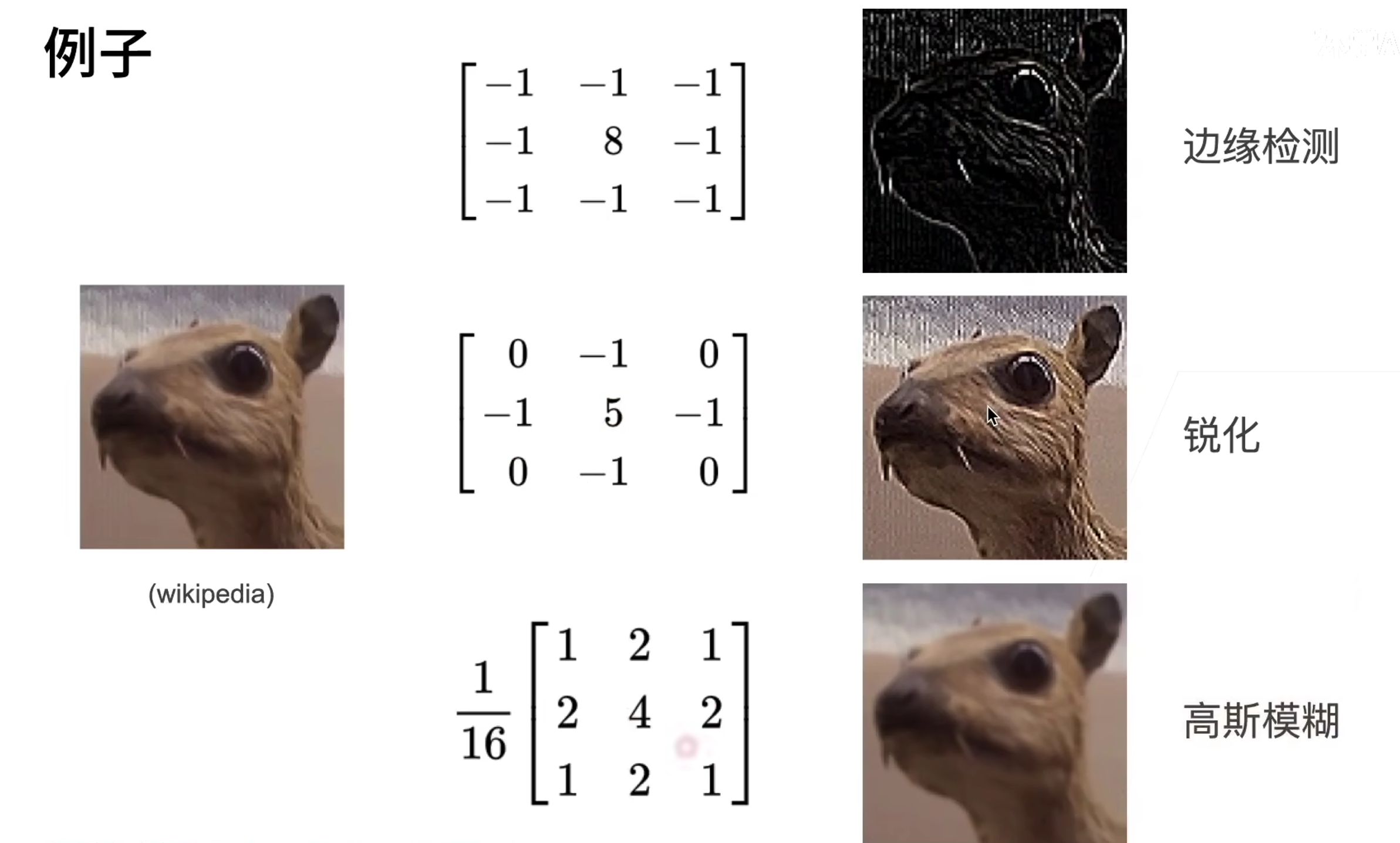
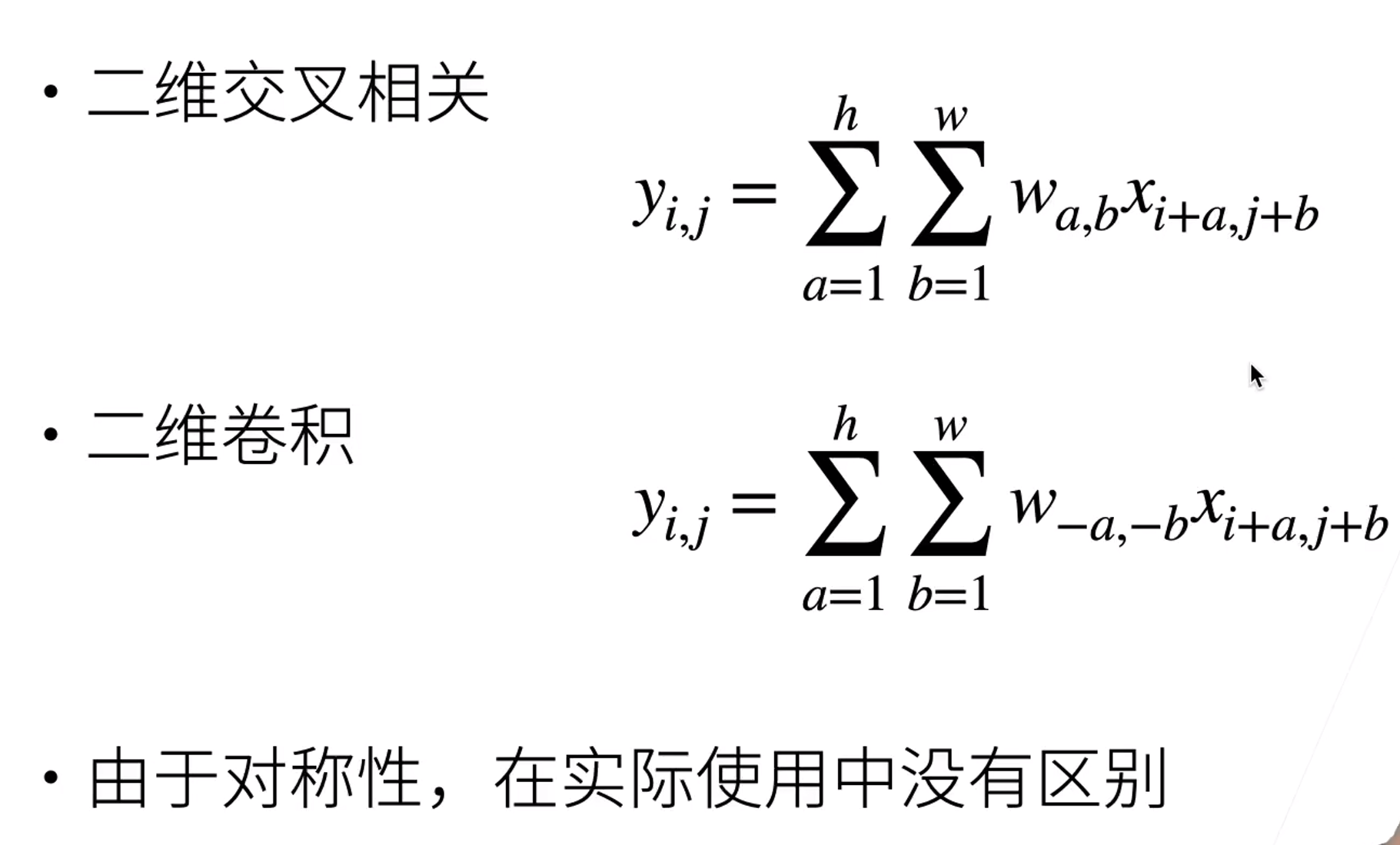
二维交叉相关
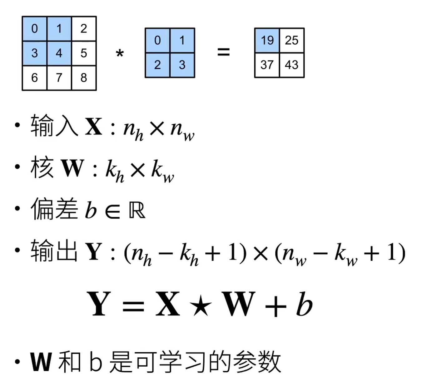
二维卷积层
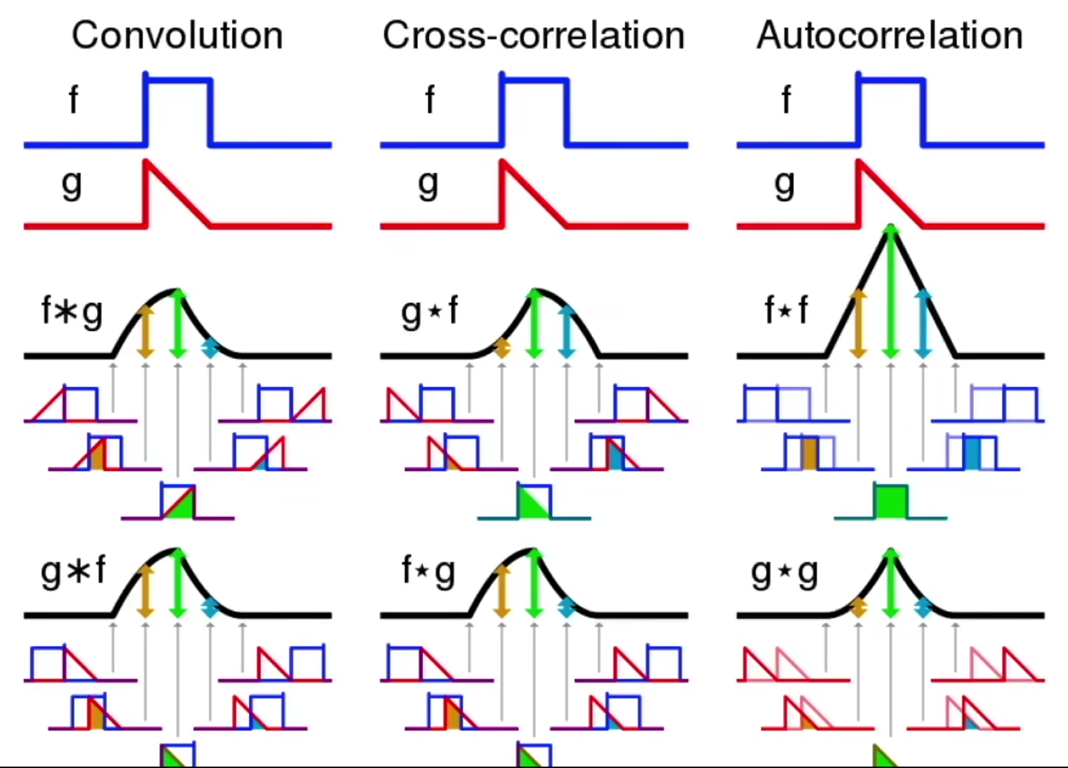
交叉相关vs卷积
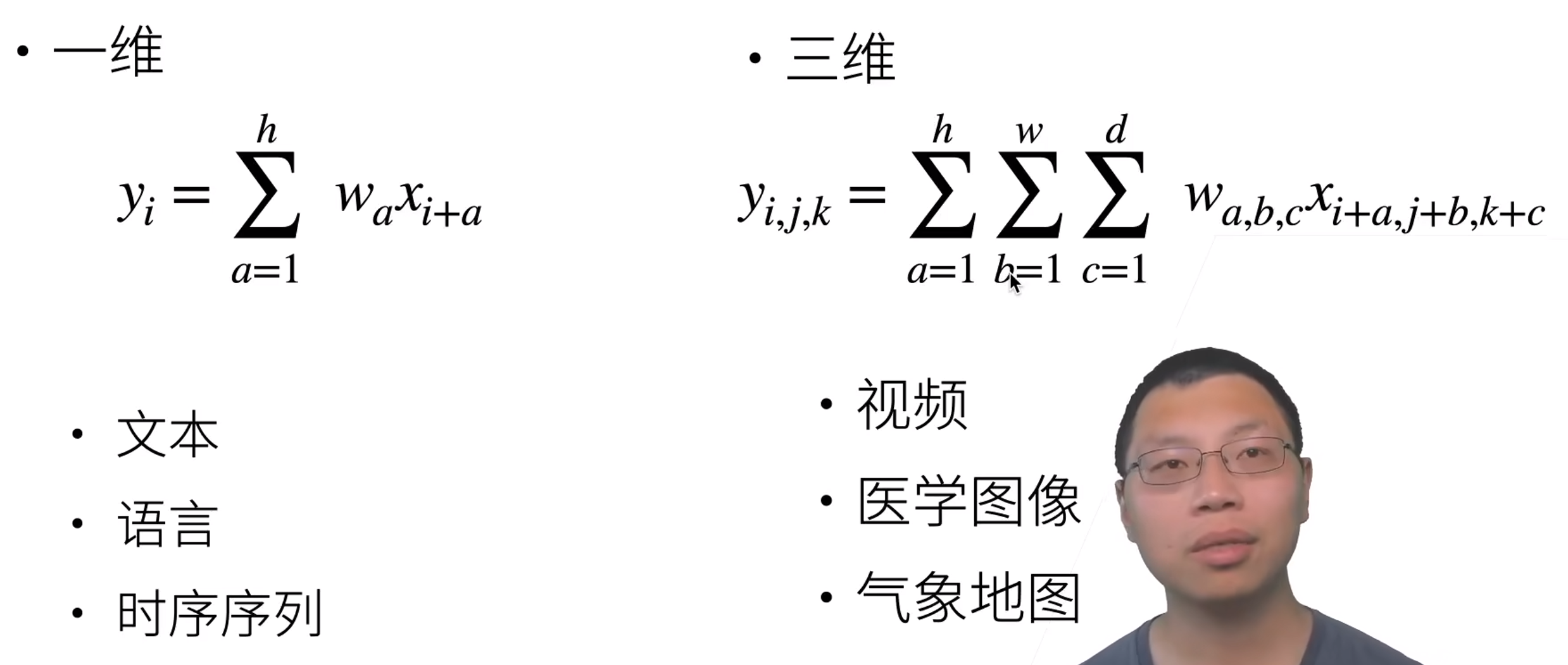
一维和三维交叉相关 总结
卷积层将输入和核矩阵进行交叉相关,加上偏移后得到输出
核矩阵和偏移是可学习的参数
核矩阵的大小是超参数
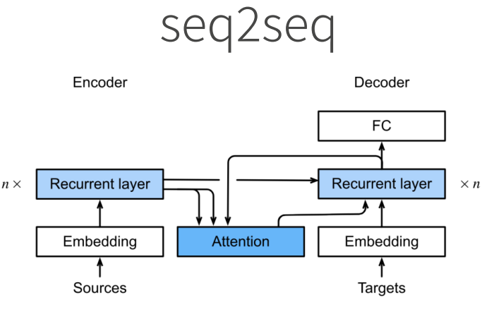
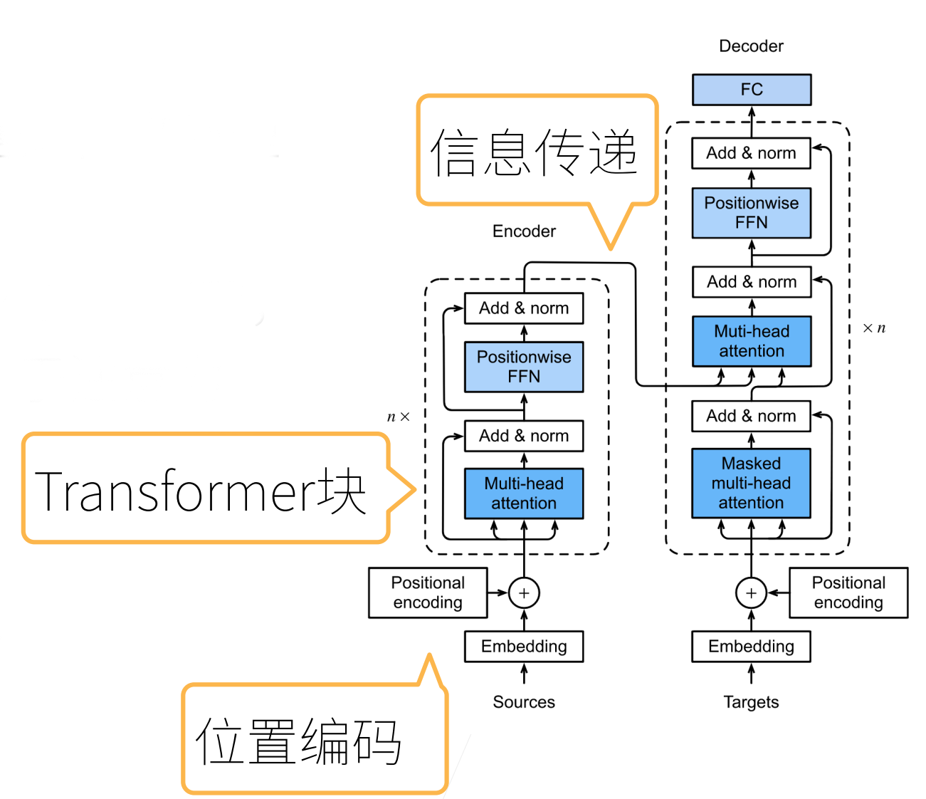
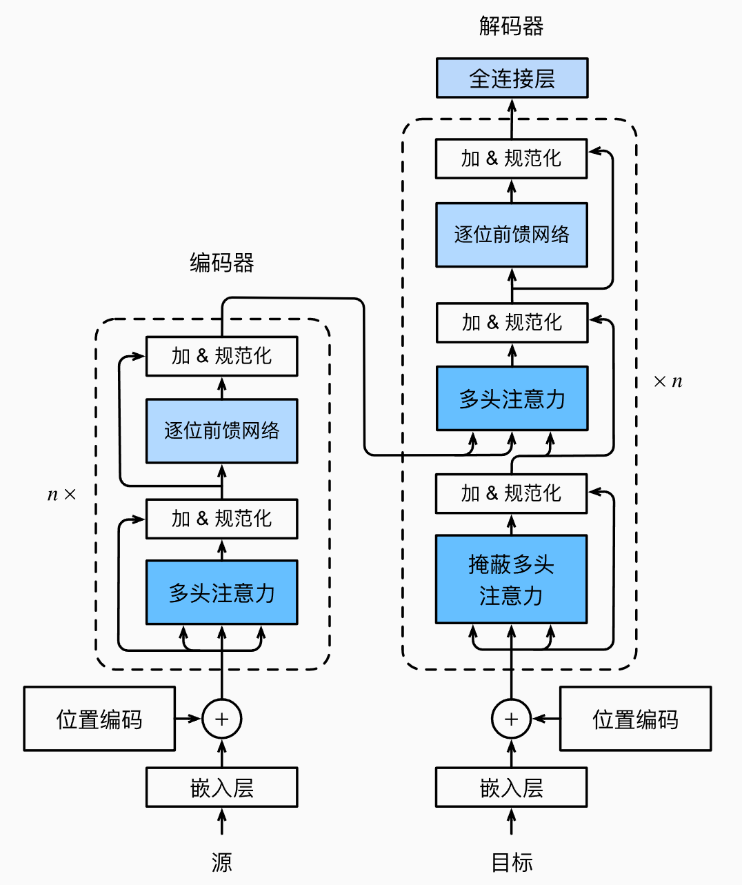
基于编码器-解码器架构来处理序列对
跟使用注意力的seq2seq不同,Transformer是纯基于注意力
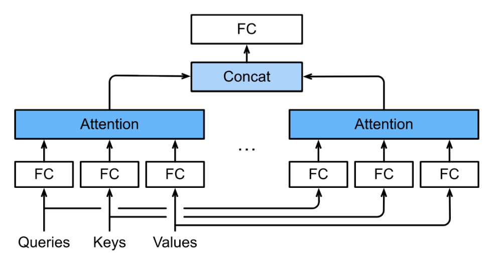
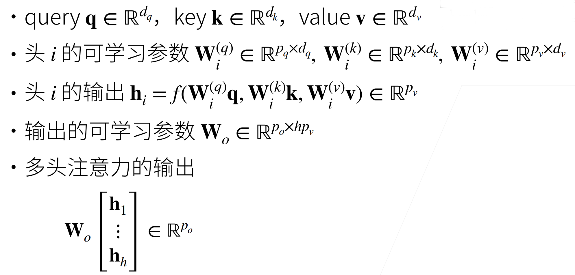
多头注意力
对同一Key,value,query,希望抽取不同的信息
多头注意力使用h个独立的注意力池化