一种新的噪声感知深度学习模型用于水声降噪
Abstract
Underwater acoustic signal denoising technology aims to overcome the challenge of recovering valuable ship target signals from noisy audios by suppressing underwater background noise. Traditional statistical-based denoising techniques are difficult to be applied effectively in complex underwater environments, especially in the case of extremely low signal-to-noise ratios (SNRs). To address these problems, we propose a noise-aware deep learning model with fullband–subband attention network (NAFSA-Net) for underwater acoustic signal denoising. NAFSA-Net adopts an encoder to extract the feature representation of the input audio. Subsequently, the noise subnet and the target subnet are designed to estimate the noise component and the target component simultaneously. Specifically, some stacked fullband–subband attention (FSA) blocks are deployed in each subnet to capture both global dependencies and fine-grained local dependencies of features. Furthermore, we introduce an interaction module to transmit auxiliary information from the noise subnet to the target subnet. Finally, we propose an improved weight scale-invariant signal-to-noise ratio (SI-SNR) loss function to optimize the training of our model. Experimental results show that our proposed NAFSA-Net substantially outperforms traditional methods and competitive DNN-based solutions in denoising underwater noisy signals with very low SNRs. More importantly, our proposals achieve equally excellent performance on both unseen datasets, which indicates that NAFSA-Net can be a more robust choice for real-world underwater acoustic denoising systems.水声信号去噪技术旨在通过抑制水下背景噪声,从噪声中恢复有价值的舰船目标信号。传统的基于小波变换的去噪技术难以有效地应用于复杂的水下环境,特别是在信噪比极低的情况下。为了解决这些问题,我们提出了一种具有全频带子带注意力网络(NAFSA-Net)的噪声感知深度学习模型,用于水声信号去噪。NAFSA网络采用编码器提取输入音频的特征表示。随后,设计噪声子网和目标子网,以同时估计噪声分量和目标分量。具体而言,在每个子网中部署一些堆叠的全频带子带注意(FSA)块,以捕获特征的全局依赖性和细粒度局部依赖性。此外,我们还引入了一个交互模块,将辅助信息从噪声子网传输到目标子网。最后,我们提出了一种改进的权重尺度不变信噪比(SI-SNR)损失函数来优化我们的模型的训练。实验结果表明,我们提出的NAFSA-Net在对具有非常低SNR的水下噪声信号进行去噪方面大大优于传统方法和基于竞争性DNN的解决方案。更重要的是,我们的建议在两个看不见的数据集上都实现了同样出色的性能,这表明NAFSA-Net可以成为现实世界水声去噪系统的更强大的选择。
Index Terms索引词
Fullband–subband attention (FSA) network, noise-aware, noise-aware deep learning model with fullband–subband attention network (NAFSA-Net), underwater acoustic denoising.全频带-子带注意力(FSA)网络,噪声感知,具有全频带-子带注意力网络的噪声感知深度学习模型(NAFSA-Net),水下声学去噪。
I. INTRODUCTION
ACCURATELY monitoring and discovering quiet surface or underwater targets have always been an exceedingly challenging task in a complex and always changing marine environment. After long-distance transmission, the acoustic signal radiated by the target will inevitably be corrupted by marine environmental noise, such as wind, rain, flow, and sounds from marine life [1]. Therefore, the underwater acoustic signals collected by hydrophones contain a large amount of worthless noise information, which brings serious challenges to the follow-up processing of underwater acoustic tasks, such as vessel recognition, positioning, and tracking [2], [3], [4], [5], [6]. Hence, it is an inherent challenge to exploit a reasonable denoising method to suppress ambient noise while retaining as much valuable information about the target audio as possible, which is the focus of this article.在复杂多变的海洋环境中,精确监测和发现水面或水下安静目标一直是一项极具挑战性的任务。目标辐射的声信号经过长距离传输后,不可避免地会受到风、雨、流、海洋生物声音等海洋环境噪声的干扰[1]。因此,水听器采集到的水声信号中含有大量无用的噪声信息,这给水声任务的后续处理,如船舶识别、定位、跟踪等带来了严峻的挑战[2],[3],[4],[5],[6]。因此,利用合理的去噪方法来抑制环境噪声,同时保留尽可能多的关于目标音频的有价值的信息是一个固有的挑战,这是本文的重点。
Generally, the sounds radiated by underwater targets are mainly composed of narrowband components (line spectrum) and wideband components (continuous spectrum) [7]. The generation of the line spectrum is mainly caused by the motion of mechanical parts and propellers, as well as the resonance of the blades. Compared with the latter, the narrowband components have higher intensity and frequency stability, which contain more important target feature information. Fig. 1(a) and (b) presents the amplitude spectra and the power spectral density (PSD) of a surface vessel. Note that the red boxes in these figures mark the main frequency and harmonic components of the ship. It can be observed that the ship audio shows five dominant line spectral features. These line spectral components are usually distributed in the lowfrequency band, with little attenuation during the propagation process. Therefore, the narrowband components of underwater target signals are usually used as an important basis for target detection and feature analysis.一般情况下,水下目标辐射的声音主要由窄带分量(线谱)和宽带分量(连续谱)组成[7]。线谱的产生主要是由机械部件和螺旋桨的运动以及叶片的共振引起的。与后者相比,窄带分量具有更高的强度和频率稳定度,包含了更重要的目标特征信息。图1(a)和(B)显示了水面船舶的振幅谱和功率谱密度(PSD)。请注意,这些图中的红框标记了船舶的主要频率和谐波分量。可以观察到,船舶音频显示出五个主导线谱特征。这些线谱分量通常分布在低频带,在传播过程中衰减很小。因此,水下目标信号的窄带分量通常被用作目标检测和特征分析的重要依据。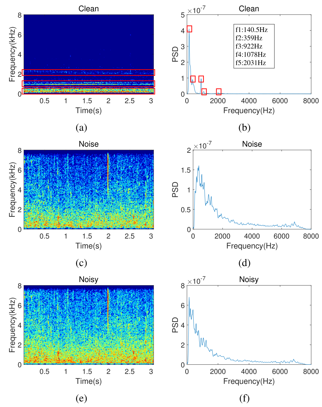
Fig. 1. T-F domain spectrograms and PSD of clean audio, noise audio, and noisy audio (−10 dB). (a) Magnitude spectra of the clean signal. (b) PSD of the clean signal. (c) Magnitude spectra of the noise signal. (d) PSD of the noise signal. (e) Magnitude spectra of the noisy signal. (f) PSD of the noisy signal.
Fig. 1.干净音频、噪声音频和噪声音频(−10 dB)的T-F域频谱图和PSD。(a)干净信号的幅度谱。(b)干净信号的PSD。(c)噪声信号的幅度谱。(d)噪声信号的PSD。(e)噪声信号的幅度谱。(f)噪声信号的PSD。
In terms of underwater acoustic signal denoising, traditional statistical prediction approaches, such as spectral subtraction [8], Wiener filtering [9], wavelet decomposition [10], empirical mode decomposition (EMD) [11], and adaptive line enhancer (ALE) [12], have been suggested, and significant progress has been made on this issue. These solutions mainly rely on the accurate analysis and modeling of the signal, as well as optimal fine-tuning of parameters. Spectral subtraction and Wiener filtering approaches are initially introduced. These methods first analyze and model the noise components in the noisy signal. Although they are simple in design and generally of low complexity, these techniques introduce additional audible spectral components after denoising, resulting in subsequent distortion of the raw audio. In addition, signal decomposition-based methods, such as wavelet decomposition and EMD, aim to decompose the noisy signal first and remove the noise components to improve the signalto-noise ratios (SNRs). The former needs to address the constraints such as optimal wavelet basis selection, threshold rule setting, and decomposition level setting, while the latter undergoes the problem of mode mixing in the EMD process. Besides, the ALE method utilizes the correlation difference between the narrowband components and the wideband components in the noisy signal to extract the line spectral features of the target signal, which has been successfully applied to passive sonar signal denoising. Unfortunately, these approaches perform poorly in quiet and remote marine scenarios. In the low SNR (−10 dB) signal, as shown in Fig. 1(e) and (f), the target signal has been completely covered by the background noise, as shown in Fig. 1(c) and (d). As the SNR continues to decrease, the performance of traditional techniques deteriorates dramatically.在水声信号去噪方面,人们提出了传统的统计预测方法,如谱减法[8]、维纳滤波[9]、小波分解[10]、经验模式分解(EMD)[11]和自适应谱线增强器(ALE)[12],并取得了显著的进展。这些解决方案主要依赖于对信号的准确分析和建模,以及参数的最佳微调。首先介绍了谱减法和维纳滤波法。这些方法首先对噪声信号中的噪声分量进行分析和建模。虽然这些技术设计简单,通常复杂度较低,但它们在去噪后引入了额外的可听频谱分量,导致随后的原始音频失真。此外,基于信号分解的方法,如小波分解和经验模式分解,其目的是首先对含噪信号进行分解,然后去除噪声成分,以提高信噪比。前者需要处理最优小波基选择、阈值规则设置、分解层设置等约束条件,而后者则需要解决EMD过程中的模式混合问题。此外,ALE方法利用噪声信号中窄带分量和宽带分量之间的相关性差异来提取目标信号的线谱特征,并已成功地应用于被动声纳信号去噪。不幸的是,这些方法在安静和偏远的海洋场景中表现不佳。在低信噪比(−10分贝)信号中,如图1(E)和(F)所示,目标信号已完全被背景噪声覆盖,如图1(C)和(D)所示。随着信噪比的不断降低,传统方法的性能急剧恶化。
Fig. 1. T-F domain spectrograms and PSD of clean audio, noise audio, and noisy audio (−10 dB). (a) Magnitude spectra of the clean signal. (b) PSD of the clean signal. (c) Magnitude spectra of the noise signal. (d) PSD of the noise signal. (e) Magnitude spectra of the noisy signal. (f) PSD of the noisy signal.
Fig. 1.干净音频、噪声音频和噪声音频(−10 dB)的T-F域频谱图和PSD。(a)干净信号的幅度谱。(b)干净信号的PSD。(c)噪声信号的幅度谱。(d)噪声信号的PSD。(e)噪声信号的幅度谱。(f)噪声信号的PSD。
Recently, data-driven methods based on deep neural networks (DNNs) have been widely used in the field of acoustic signals and have been proven to be effective and outperform conventional solutions in solving audio denoising problems. The mainstream DNN-based methods can be classified into two categories: the time–frequency (T-F) domain denoising methods [13], [14], [15], [16] and the time-domain denoising methods [17], [18], [19], [20]. The T-F domain methods operate signals on the T-F spectrogram. These schemes first convert the audio waveform to T-F spectrogram by short-time Fourier transform (STFT) and then predict a weighing mask between the noisy signal and the target clean signal [21], [22], [23] or directly estimate the spectral representations of clean signals [24], [25], [26]. Unlike the former, the time-domain denoising methods directly estimate the clean audio waveform from the raw time-domain signal in an end-to-end way. Most of the aforementioned methods have a salient feature of utilizing the clean signal as the training target. However, in the low SNR scenarios, the weak-energy target signal components are nearly buried in the noisy signal in which noise components dominate. In this case, it becomes prohibitively difficult to directly predict the clean signal from the pure-noise-like noisy signal.近年来,基于深度神经网络(DNN)的数据驱动方法在声信号领域得到了广泛的应用,在解决音频去噪问题上被证明是有效的并且优于传统的解决方案。目前主流的基于离散神经网络的去噪方法可以分为两类:时频(T-F)域去噪方法[13]、[14]、[15]、[16]和时间域去噪方法[17]、[18]、[19]、[20]。T-F域法对T-F谱图上的信号进行运算。这些方案首先通过短时傅里叶变换(STFT)将音频波形转换为T-F谱图,然后预测噪声信号和目标清洁信号[21]、[22]、[23]之间的加权掩码或直接估计清洁信号[24]、[25]、[26]的谱表示。与前者不同的是,时域去噪方法直接从原始的时域信号中端到端地估计出干净的音频波形。大多数前述方法的显著特征是利用CLEAN信号作为训练目标。然而,在低信噪比的情况下,微弱能量的目标信号分量几乎被淹没在噪声分量占主导地位的噪声信号中。在这种情况下,从纯噪声类噪声信号中直接预测清洁信号变得非常困难。
To address the above problem, a novel noise-aware deep learning model with fullband–subband attention network (NAFSA-Net) is proposed to perform denoising of ship radiation signals, in which the noise signal and the target signal are estimated simultaneously through different subnets. In addition, we deploy an information interaction module between the two subnets, by which the noise subnet transmits complementary information to the target subnet and guides the training of the latter in obtaining additional noise-like, weak-energy target information. Taking this as an advantage, we exploit an improved weighted scale-invariant signalto-noise ratio (SI-SNR) loss function, namely, iwSI-SNR, to guide the training of the network. In addition, the spectral characteristics of ship signals inspire the assumption that valuable feature information is concentrated in the specific narrow-band regions and that ship engine sound has a distinct spatio-temporal distribution in the T-F domain. Fullband– subband attention (FSA) blocks are developed to aggregate context dependencies, in which channel attention is utilized to model fullband correlation and subband attention is used to extract the fine-grained short-term dependencies.为了解决上述问题,提出了一种新的噪声感知深度学习模型--全频带子带注意力网络(NAFSA-Net),用于对舰船辐射信号进行去噪,该模型通过不同的阈值同时估计噪声信号和目标信号。此外,我们部署了一个信息交互模块之间的两个子网,通过该噪声子网传输补充信息的目标子网,并指导后者的训练,以获得额外的噪声类,弱能量的目标信息。以此为优势,我们利用改进的加权尺度不变信噪比(SI-SNR)损失函数,即iwSI-SNR,来指导网络的训练。此外,船舶信号的频谱特性激发了这样的假设,即有价值的特征信息集中在特定的窄带区域,并且船舶发动机声音在T-F域中具有独特的时空分布。提出了全频带子带注意(FSA)模块来聚合上下文相关性,其中信道注意用于建模全频带相关性,子带注意用于提取细粒度的短期相关性.
The rest of this article is organized as follows. We provide a detailed analysis of related work in Section II. Section III explains the overall architecture and important components of NAFSA-Net. In Section IV, we introduce the experimental procedures. Next, we extensively evaluate the performance of the proposal and discuss the results in Section V. Finally, we conclude this article in Section VI.本文的其余部分组织如下。我们在第二节中对相关工作进行了详细的分析。第三节解释了北美渔业安全网的总体结构和重要组成部分。在第四节中,我们介绍了实验程序。接下来,我们在第五节中广泛评估了该提案的性能并讨论了结果。最后,我们在第六节中总结了这篇文章。
II. RELATED WORK
A. Deep Neural Network-Based Audio DenoisingA.基于深度神经网络的音频去噪
In general, DNN-based denoising schemes mainly build the mapping model from mixed audio to target audio by training and learning on a large amount of data. Benefiting from powerful nonlinear modeling capabilities, such methods have shown remarkable superiority over traditional solutions. Two typical DNN-based denoising frameworks are shown in Fig. 2.通常,基于DNN的去噪方案主要通过对大量数据的训练和学习来建立从混合音频到目标音频的映射模型。由于其强大的非线性建模能力,这些方法已经显示出明显优于传统的解决方案。两个典型的基于DNN的去噪框架如图2所示。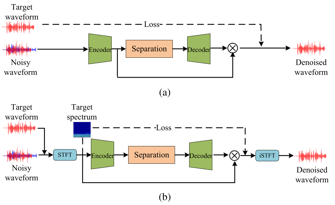
Fig. 2. Illustration of different audio denoising frameworks. (a) Block diagram of the time-domain audio denoising framework. (b) Block diagram of the T-F domain audio denoising framework.
图二 不同音频去噪框架的插图。(a)时域音频去噪框架的框图。(b)T-F域音频去噪框架的框图。
Given a target signal s and a noise signal n, the noisy audio can be defined as给定目标信号s和噪声信号n,噪声音频可以被定义为:
where m ∈ 1, . . . , M, {x, s, n} ∈ RM×1, and M represents the number of samples in the signal. Fig. 2(a) shows the standard block diagram of the time-domain denoising framework. We can formulate the DNN-based denoising in the time domain as其中m∈1,.。。,M,{x,S,n}∈Rm×1,M表示信号中的采样数。图2(A)示出了时间域去噪框架的标准框图。我们可以将基于DNN的时间域去噪表示为
where θ represents the parameter of neural network and sˆ is the denoised target signal. In the training phase, raw waveforms are directly fed into the denoising model. Timedomain methods model noisy waveforms and recover clean waveforms via a learnable encoder–decoder network.其中,θ表示神经网络的参数,并且s θ是去噪后的目标信号。在训练阶段,原始波形被直接馈送到去噪模型中。时域方法对噪声波形进行建模,并通过可学习的编码器-解码器网络恢复干净的波形。
Different from the former, T-F domain methods first convert the audio to the T-F domain by STFT, and the corresponding spectral representations in the T-F domain can be described as与前者不同的是,T-F域方法首先通过STFT将音频转换到T-F域,并且T-F域中相应的频谱表示可以被描述为
Note that {X, S, N} ∈ R^(F×T) denote the complex-valued T-F representation of noisy audio, target audio, and noise audio, respectively. T denotes the total number of time frames, and F is the number of frequency bins. A block diagram of the T-F domain denoising framework is shown in Fig. 2(b). T-F domain methods take spectrogram as an input feature to the network. Such methods typically predict a weighting mask to map from noisy T-F representation to clean T-F representation or directly estimate the target spectrum. Finally, inverse STFT (iSTFT) is used to reconstruct the denoised waveform.请注意,{X,S,N}∈R^(F×T) 分别表示噪声音频、目标音频和噪声音频的复值T-F表示。T表示时间帧的总数,而F表示频率段的数目。图2(B)显示了T-F域去噪框架的框图。T-F域法将谱图作为网络的输入特征。这种方法通常预测加权掩码以从噪声的T-F表示映射到干净的T-F表示,或者直接估计目标频谱。最后,利用逆短时傅立叶变换(ISTFT)重构去噪后的波形。
Although DNN-based audio denoising techniques have shown considerable improvements compared with traditional model-based approaches, they only model the target signal, ignoring the importance of noise knowledge. What is more, these methods are mostly applied under relatively high SNR conditions and are not adapted for low SNR underwater target data.虽然基于DNN的音频去噪技术与传统的基于模型的方法相比已经显示出相当大的改进,但它们只对目标信号进行建模,忽略了噪声知识的重要性。而且这些方法大多适用于信噪比较高的情况,不适合低信噪比的水下目标数据。
B. Noise-Aware Audio DenoisingB.噪声感知音频去噪
Traditional denoising methods usually achieve noise reduction by first estimating noise information [27], [28], [29]. For instance, spectral subtraction and Wiener filtering methods use silent segments of audio to gain noise distribution knowledge and then enhance the target audio. However, the ship-radiated audio is different from the speech signal, the former is persistent in the noisy signal, and there are no silent segments. Therefore, it is very challenging to accurately estimate the PSD of underwater nonstationary noise, which is usually assumed to be stationary. This assumption limits the upper bound on the performance of denoising methods.传统的去噪方法通常通过首先估计噪声信息来实现降噪[27],[28],[29]。例如,谱减法和维纳滤波方法使用音频的静音段来获得噪声分布知识,然后增强目标音频。然而,船舶辐射音频不同于语音信号,前者在噪声信号中是持久的,并且不存在无声段。因此,它是非常具有挑战性的准确估计的功率谱的水下非平稳噪声,这通常是假定为平稳的。这种假设限制了去噪方法性能的上限。
DNN-based methods are data-driven and avoid artificial errors introduced by inaccurate assumptions. Researchers have made many beneficial attempts on incorporating noise knowledge when estimating target audio. The most straightforward solution is to add constraints on noise information to the loss function [30], [31], [32]. Such approaches do not model noise, and the estimation of the target signal acquires little gain from prior knowledge of the noise. In addition, Odelowo and Anderson [33] propose a noise prediction scheme to handle the speech enhancement task, which directly estimates noise instead of the clean target audio. This method lacks target information and even underperforms classical target-aware methods at low SNR conditions and in unseen noise scenarios. Sun et al. [34] propose a separable deep autoencoder (DAE) to estimate noise for assisting target signal enhancement. This method trains DAE networks in two stages to model target audio and noise audio separately with the constraint that the sum of the outputs of the two DAEs is equal to the noisy audio. In this article, we introduce a noise-aware network to model target and noise audio simultaneously. The noise subnet is trained to assist target audio enhancement by transmitting embedding auxiliary knowledge to the target subnet through several interaction modules. This scheme makes it suitable for low SNR conditions.基于DNN的方法是数据驱动的,避免了由不准确的假设引入的人为错误。研究人员在估计目标音频时结合噪声知识进行了许多有益的尝试。最直接的解决方案是将对噪声信息的约束添加到损失函数[30],[31],[32]。这样的方法不对噪声建模,并且目标信号的估计从噪声的先验知识获得很少的增益。此外,Odelowo和安德森[33]提出了一种噪声预测方案来处理语音增强任务,该方案直接估计噪声而不是干净的目标音频。该方法缺乏目标信息,甚至在低信噪比条件下和不可见噪声场景下的性能低于经典的目标感知方法。Sun等人。[34]提出了一种可分离的深度自动编码器(DAE)来估计噪声,以辅助目标信号增强。该方法分两个阶段训练DAE网络,分别对目标音频和噪声音频进行建模,约束条件是两个DAE的输出之和等于噪声音频。在这篇文章中,我们介绍了一种噪声感知网络,可以同时对目标和噪声音频进行建模。训练噪声子网,通过多个交互模块向目标子网传输嵌入辅助知识来辅助目标音频增强。该方案使其适用于低SNR条件。
C. Attention-Based ModelC.注意力模型
The attention mechanism is first introduced to solve sequence-to-sequence tasks, such as machine translation [35] and speech recognition [36]. It was subsequently expanded into the field of computer vision [37], [38], [39], [40] and audio signal processing [19], [41], [42] with great success. Pandey and Wang [19] propose a dense convolutional network with self-attention for speech enhancement, where the attention module is designed to capture utterance level dependencies. Besides, researchers suggest using channelwise attention along the frequency dimension of the complex-valued spectrum to capture the structural features of the signal [15], [43]. In the aforementioned approaches, the attention mechanism is typically applied together to capture global context aggregation along the time dimension or frequency dimension. Different from previous solutions, we suggest using fullband attention and subband attention to capture long- and short-term features, respectively, so as to better recover the weak line spectrum part of the ship signal. It is worth noting that each attention block captures dependencies from two dimensions, time and frequency, respectively. Such attention blocks are employed in both the target subnet and noise subnet.注意力机制首先被引入来解决序列到序列的任务,例如机器翻译[35]和语音识别[36]。它随后扩展到计算机视觉领域[37],[38],[39],[40]和音频信号处理[19],[41],[42]并取得了巨大成功。Pandey和Wang [19]提出了一种用于语音增强的具有自注意力的密集卷积网络,其中注意力模块旨在捕获话语级别依赖性。此外,研究人员建议沿着复值频谱的频率维度使用通道注意力来捕获信号的结构特征[15],[43]。在上述方法中,注意力机制通常被一起应用以沿着时间维度或频率维度捕获全局上下文聚合。与以往的解决方案不同,我们建议使用全带注意和子带注意,分别捕获长期和短期的功能,以便更好地恢复船舶信号的弱线谱部分。值得注意的是,每个注意力块分别从时间和频率两个维度捕获依赖关系。在目标子网和噪声子网中都采用这样的注意力块。
III. NOISE-AWARE SUBBAND ATTENTION NETWORK
三.噪声感知子带注意网络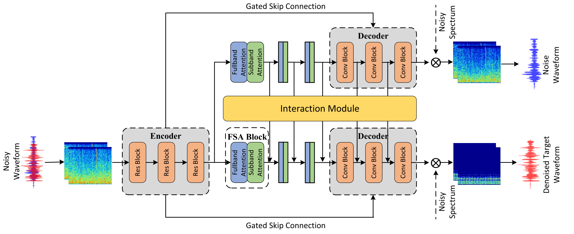
Fig. 3. Overall network architecture of the proposed NAFSA-Net.
图3 拟议的NAFSA网络的总体网络架构。
Fig. 3 presents the overall network architecture of the proposed NAFSA-Net. The main building blocks of NAFSA-Net are the encoder–decoder module, the FSA blocks, and the interaction module. Our model takes the STFT-transformed complex-valued spectrum as input, and the input feature can be denoted as X ∈ R^(F×T×2). Subsequently, the encoder extracts the feature representations of the original signal and feeds them into the noise and target subnets. To take full advantage of the prior feature differences between noise and target on the T-F spectrogram, several stacked FSA blocks are deployed in different subnets for exploiting the dependencies of the noise and target components, respectively. Then, the decoder receives information from the encoder and FSA blocks to reconstruct the complex-valued spectrum corresponding to each subnet. In NAFSA-Net, an interaction module is introduced to transfer supplementary information from the noise subnet to the target subnet. In this way, the target subnet is expected to obtain complementary information. Finally, the denoised spectrum is converted back to the waveform by iSTFT.图3显示了所提出的NAFSA网络的整体网络架构。NAFSA-Net的主要构建块是编码器-解码器模块、FSA块和交互模块。我们的模型以STFT变换后的复值谱作为输入,输入特征可以表示为 X ∈ R^(F×T×2)。随后,编码器提取原始信号的特征表示,并将其馈送到噪声和目标噪声中。为了充分利用T-F谱图上噪声和目标之间的先验特征差异,将几个堆叠的FSA块部署在不同的频带中,以分别利用噪声和目标分量的依赖性。然后,解码器从编码器和FSA块接收信息以重构对应于每个子网的复值频谱。在NAFSA网络中,引入了一个交互模块,将补充信息从噪声子网传输到目标子网。以这种方式,期望目标子网获得补充信息。最后,通过iSTFT将去噪频谱转换回波形。
A. Encoder and Decoder ModuleA.编码器和解码器模块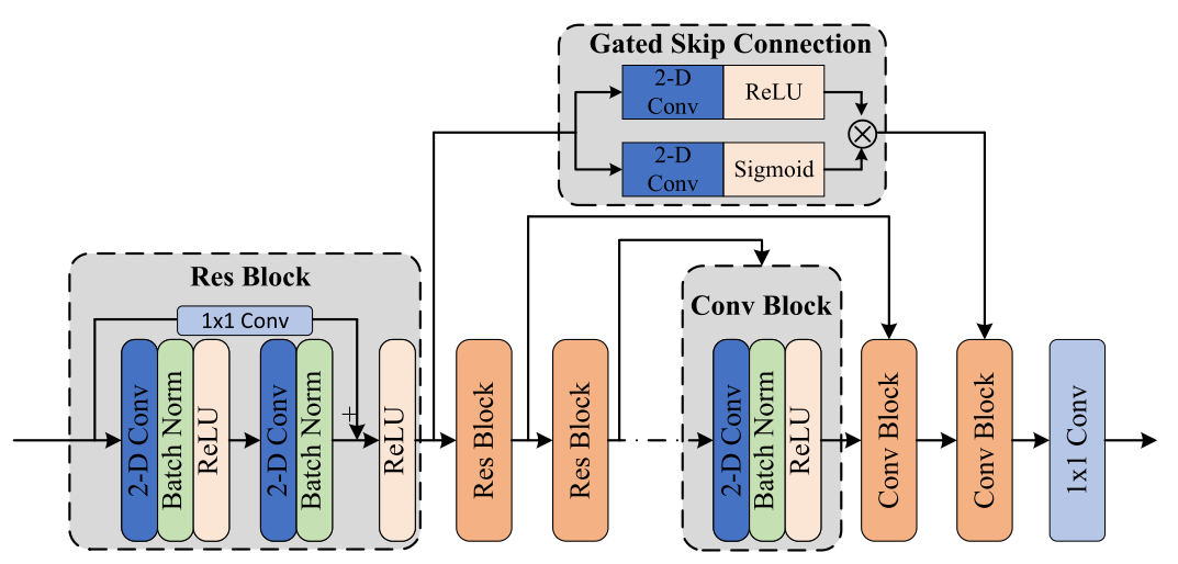
Fig. 4. Encoder–decoder module. The dashed arrow indicates the separation part with FSA blocks.
图4 编码解码器模块。虚线箭头指示具有FSA块的分离部分。
In NAFSA-Net, the noise subnet and the target subnet share the encoder part. Fig. 4 illustrates the encoder–decoder-based architecture of NAFSA-Net. Three modified residual blocks are introduced in the encoder to extract latent features from spectral features. Each modified residual block consists of two 2-D convolutional layers with a kernel size of (5, 7) and a stride of (1, 1). Different from the traditional residual block, the number of channels in the convolutional layer will increase relative to their inputs. Moreover, a 1×1 convolutional layer is deployed in the skip connection part to maintain the consistency of residual inputs. All the convolutional layers in the encoder are followed by batch normalization (BN) and a rectified linear unit (ReLU). Note that we use D^(enc) ∈ R^(F×T×C) to denote the outputs of the encoder, where C is the channel number. The number of output channels for each block is 6, 12, and 24, respectively. In order to maintain sufficient resolution, no downsampling is performed in the time and frequency dimensions of the features.在NAFSA网络中,噪声子网和目标子网共享编码器部分。图4示出了NAFSA网络的基于编码器-解码器的架构。在编码器中引入了三个改进的残差块,以从谱特征中提取潜在特征。每个修改后的残差块由两个2-D卷积层组成,其内核大小为(5,7),步幅为(1,1)。与传统的残差块不同,卷积层中的通道数量将相对于其输入增加。此外,在跳过连接部分部署了1×1卷积层,以保持剩余输入的一致性。编码器中的所有卷积层后面都是批量归一化(BN)和整流线性单元(ReLU)。注意,我们使用D^(enc) ∈ R^(F×T×C)来表示编码器的输出,其中C是通道数。每个块的输出通道数分别为6、12和24。为了保持足够的分辨率,在特征的时间和频率维度中不执行下采样。
As shown in Fig. 4, the decoder contains three consecutive convolution blocks followed by a 1 × 1 convolution layer, which learns the complex ratio mask of noise and target audio, and denoted by如图4所示,解码器包含三个连续的卷积块,后面是1 × 1卷积层,它学习噪声和目标音频的复比掩码,并表示为
and
respectively.
Each Conv block receives the output of the previous module and the output of the corresponding residual block in the encoder. All the 2-D convolution layers are followed by a ReLU activation and a BN layer. The kernel size and stride for all 2-D convolution layers are set to (1, 1) and (1, 1). The channel numbers are 12, 6, and 2, respectively. In particular, we propose to use gated convolution [44] instead of a direct skip connection to filter the feature information from the encoder to different subnets.每个Conv块接收先前模块的输出和编码器中的对应残差块的输出。所有的二维卷积层之后都是ReLU激活和BN层。所有2-D卷积层的内核大小和步幅设置为(1,1)和(1,1)。频道号分别为12、6和2。特别是,我们建议使用门控卷积[44]而不是直接跳过连接来过滤来自编码器的特征信息到不同的编码器。
B. Fullband–Subband Attention BlockB.全频带-子频带注意阻断
NAFSA-Net captures dependencies by aggregating fullband attention and subband attention. In this section, we first introduce the implementation of fullband attention via channel adaptive strategy and subband attention via the sliding window, respectively. After that, we present the aggregating strategy of the FSA block.NAFSA网络通过聚合全频带注意力和子带注意力来捕获依赖关系。在这一节中,我们首先介绍了通过信道自适应策略实现全带注意和通过滑动窗口实现子带注意。在此基础上,提出了FSA模块的聚合策略。
1)Fullband Attention via Channel Adaptive Strategy: Different vessels usually exhibit unique frequency band distribution characteristics in the spectrogram. In addition, valuable frequency and harmonic components of the ship tend to concentrate in the lower frequency band of mixed audio. Also, inspired by the successful application of channelwise attention in computer vision [45], [46], we propose to capture the global distribution characteristics of spectrogram by fullband attention via channel adaptive strategy. This scheme takes the frequency dimension as the channel dimension of the channel attention mechanism, which adaptively learns a weight vector corresponding to each frequency bin based on the spectral feature information. The proposed fullband attention is shown in Fig 5.1)通过通道自适应策略实现全频带注意:不同的血管通常在频谱图中表现出独特的频带分布特征。此外,船舶的有价值的频率和谐波分量往往集中在混合音频的较低频带。此外,受通道注意力在计算机视觉中的成功应用的启发[45],[46],我们提出通过通道自适应策略通过全带注意力来捕获谱图的全局分布特征。该方案将频率维度作为信道关注机制的信道维度,根据频谱特征信息自适应地学习每个频率点对应的权向量。所提出的全频带注意力如图5所示。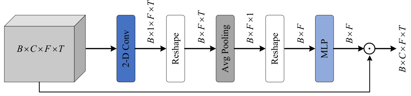
Fig. 5. Diagram of fullband attention.
图五 全波段注意力示意图。
Given an intermediate feature D with the shape of B × C × F × T, where B denotes the batch size, first, a 2-D convolution layer is used to combine the features of multiple channels and obtain the intermediate result with the shape of B × F × T by reshape operation. Next, we aggregate the information at each frequency bin by average pooling. The reshaped features (R^(B×F)) are then fed into the MLP layer to generate the weight vector ω ∈ R^(B×F). Finally, we conduct an elementwise multiplication on the original feature D with ω after broadcasting to obtain the output (D^full ∈ R^(B×C×F×T)) of fullband attention.给定一个形状为B × C × F × T的中间特征D,其中B表示批量大小,首先,使用二维卷积层将多个通道的特征进行组合,并通过整形操作获得形状为B × F × T的中间结果。接下来,我们通过平均池化来聚合每个频率点处的信息。然后将整形后的特征(R^(B×F))馈送到MLP层以生成权重向量ω ∈ R^(B×F)。最后,我们在广播后对原始特征D与ω进行逐元素乘法,以获得全频带注意力的输出(D^full ∈ R^(B×C×F×T))。
2)Subband Attention via Sliding Window: We use a sliding window mechanism to design subband attention, which is applied to capture fine-grained correlations within local patterns of the spectrogram. Similar strategies have been employed in [47] and [48]. Specifically, the input feature maps are first decomposed into disjoint fragments with a window length of w. Each token within a local fragment attends to all tokens within its home fragment, as well as d consecutive adjacent tokens on the left and right side, yielding a local subband of total length w + 2d tokens. d indicates the length of adjacent tokens on each side. Then, we perform self-attention on all N subbands to extract short term dependencies. After that, a 2-D convolution layer is utilized to map the subbands back to home fragments of length w and ultimately generate the output of the subband attention D^sub. For boundary tokens, the zero-padding strategy proposed in [47] is applied.2)通过滑动窗口的子带注意:我们使用滑动窗口机制来设计子带注意,它被应用于捕获频谱图的局部模式内的细粒度相关性。在[47]和[48]中采用了类似的策略。具体地,输入特征图首先被分解成具有窗口长度w的不相交片段。本地片段内的每个令牌涉及其归属片段内的所有令牌,以及左侧和右侧的d个连续相邻令牌,从而产生总长度为w + 2d个令牌的本地子带。d表示每一侧上相邻标记的长度。然后,我们对所有N个子带执行自注意以提取短期依赖性。之后,利用2-D卷积层将子带映射回长度为w的归属片段,并最终生成子带关注D^sub的输出。对于边界令牌,应用[47]中提出的零填充策略。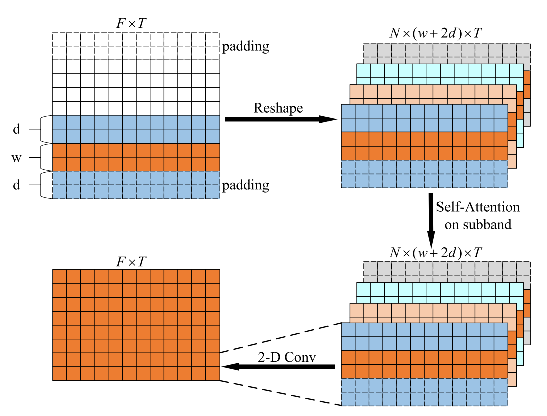
Fig. 6. Diagram of subband attention.
图6 子带注意图。
Fig. 6 illustrates the details of subband attention. Given an input feature D ∈ R^(F×T), the subband attention can be defined as图6示出了子带关注的细节。给定输入特征D ∈ R^(F×T),子带注意力可以定义为: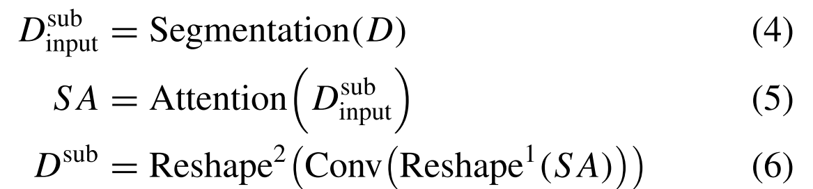
where $D_{\text {input }}^{\text {sub }} \in \mathbb{R}^{N \times F^{\text {sub }} \times T}$(N indicates the number of local subbands, and $F^{\text {sub }}=w+2 d$ represents the width of each subband, which is equal to the length of the sliding window plus the length of the extended left and right neighbors). Segmentation(·) divides feature tensors into local fragments and reorganizes them into a new feature tensor. $\operatorname{Reshape}^1(\cdot)$ denotes a vector reshape from $\mathbb{R}^{N \times F^{\text {sub }} \times T}$ to $\mathbb{R}^{F^{\mathrm{sub}} \times N \times T}$, and $\operatorname{Reshape}^2(\cdot)$ reshapes a tensor from $\mathbb{R}^{N \times w \times T}$ back to $\mathbb{R}^{F \times T}$.其中,$D_{\text {input }}^{\text {sub }} \in \mathbb{R}^{N \times F^{\text {sub }} \times T}$(N表示局部子带的数量,$F^{\text {sub }}=w+2 d$表示每个子带的宽度,其等于滑动窗口的长度加上扩展的左右邻居的长度)。分割(·)将特征张量划分为局部片段,并将它们重组为新的特征张量。$\operatorname{Reshape}^1(\cdot)$表示从$\mathbb{R}^{N \times F^{\text {sub }} \times T}$到$\mathbb{R}^{F^{\mathrm{sub}} \times N \times T}$的向量整形,$\operatorname{Reshape}^2(\cdot)$将张量从$\mathbb{R}^{N \times w \times T}$整形回$\mathbb{R}^{F \times T}$。
In the above equations, Conv(·) denotes the 2-D convolution layer with a kernel size of (1, 1) and a stride of (1, 1). A BN and a PReLU activation are added after the convolution layer. In addition, we set the length d of adjacent tokens within the subband to be equal to the window length w. The hyperparameter w will be optimized by comparative experiments.在上面的等式中,Conv(·)表示具有核大小(1,1)和步幅(1,1)的2-D卷积层。在卷积层之后添加BN和PReLU激活。此外,我们将子带内的相邻令牌的长度d设置为等于窗口长度w。超参数w将通过比较实验进行优化。
3)FSA Block: FSA blocks are deployed between the encoder and the decoder for extracting spectral features from the noise subnet and the target subnet, respectively. Each FSA block consists of two main components: fullband attention and subband attention. The former applies channelwise attention in the frequency dimension to aggregate global dependencies of input features. Different from fullband attention, the latter performs fine-grained subband attention along the frequency and time dimensions in parallel. The fine-grained attention mechanism in the frequency dimension allows the network to pay attention to the high-power narrowband spectral components. When it comes to the time dimension, the subband attention captures dependencies within local time segments, corresponding to the temporal persistence and periodicity of ship propeller sounds.3)FSA模块:FSA块部署在编码器和解码器之间,用于分别从噪声子网和目标子网中提取频谱特征。每个FSA块由两个主要部分组成:全带注意和子带注意。前者在频率维度上应用通道注意力来聚合输入特征的全局依赖性。与全带注意不同,后者并行地沿频率和时间维度执行细粒度子带注意沿着。频率维度的细粒度注意机制允许网络关注高功率窄带频谱分量。当涉及到时间维度时,子带注意力捕获本地时间段内的依赖性,对应于船舶螺旋桨声音的时间持久性和周期性。
Fig. 7. Illustration of the FSA block. Here, each FSA block first performs fullband attention on the frequency dimension of the input features. Then, subband attention is applied in parallel along the frequency and time dimensions of the input features to produce corresponding output features D^Freq and D^Time, respectively. Finally, the FSA block combines the original features D^Res with them to get the final output features.
图7 FSA块的图示。这里,每个FSA块首先对输入特征的频率维度执行全频带关注。然后,沿着输入特征的频率和时间维度并行地应用子带注意,以分别产生对应的输出特征D^Freq和D^Time。最后,FSA块将原始特征D^Res与它们组合以获得最终输出特征。
Fig. 7 shows an illustration of the FSA block. The spectral features D ∈ $\mathbb{R}^{C \times F \times T}$ are first fed into the fullband attention module to generate the intermediate features with a shape of C × F × T. To reduce computational complexity, we propose a 2-D convolution layer to halve the number of channels. The output features are then fed parallelly into a temporal subband attention and a frequencywise subband attention module. The dimensions of the input features for each of the two subband attention are $\mathbb{N}^{F}$ × $\mathbb{Subband}^{F}$ × (TC/2) and $\mathbb{N}^{T}$ × $\mathbb{Subband}^{T}$ × (FC/2), respectively. $\mathbb{N}^{k}$ , k ∈ {F, T} denotes the number of subband fragments, and $\mathbb{Subband}^{k}$ = w + 2d, k ∈ {F, T} indicates the width of local subband. We concatenated the feature $\mathbb{D}^{Freq}$ ∈ $\mathbb{R}^{(C/2) \times F \times T}$ generated by frequencywise subband attention, the feature $\mathbb{D}^{Time}$ ∈ $\mathbb{R}^{(C/2) \times F \times T}$ produced by temporal subband attention, and the residual feature $\mathbb{D}^{Res}$ ∈ $\mathbb{R}^{(C/2) \times F \times T}$. The combined features are fed into another 2-D convolution layer. Finally, the output features of the FSA block in the target subnet are fused with the information of the noise subnet passed through the interaction module, used in the subsequent modules.图7示出了FSA块的图示。首先将频谱特征D ∈ $\mathbb{R}^{C \times F \times T}$输入到全频带注意模块中,以生成具有C × F × T形状的中间特征。为了降低计算复杂度,我们提出了一个2-D卷积层,以减少一半的通道数量。然后将输出特征连续地馈送到时间子带注意和频率子带注意模块中。两个子带注意中的每一个的输入特征的维度分别为$\mathbb{N}^{F}$ × $\mathbb{Subband}^{F}$ ×(TC/2)和$\mathbb{N}^{T}$ × $\mathbb{Subband}^{T}$ ×(FC/2)。$\mathbb{N}^{k}$,k ∈ {F,T}表示子带片段的数量, $\mathbb{Subband}^{k}$ = w + 2d,k ∈ {F,T}表示局部子带的宽度。我们将由频率子带注意产生的特征$\mathbb{D}^{Freq}$ ∈ $\mathbb{R}^{(C/2) \times F \times T}$由时间子带注意产生的特征$\mathbb{D}^{Time}$ ∈ $\mathbb{R}^{(C/2) \times F \times T}$和残差特征$\mathbb{D}^{Res}$ ∈ $\mathbb{R}^{(C/2) \times F \times T}$串联起来。组合的特征被馈送到另一个2-D卷积层。最后,将目标子网FSA模块的输出特征与经过交互模块的噪声子网信息进行融合,用于后续模块。
All the convolution layers in the FSA blocks are followed by a BN and a parametric ReLU (PReLU) activation. They have the same kernel size of (1, 1) and the stride of (1, 1).FSA块中的所有卷积层后面都是BN和参数ReLU(PReLU)激活。它们具有相同的内核大小(1,1)和步幅(1,1)。
C. Interaction ModuleC.交互模块
In NAFSA-Net, the noise subnet is not independent of the target subnet, and we expect the former to enhance the training process of the latter. The noise component dominates the noisy audio with low SNR, and there are many overlapping parts of noise and ship audio in the spectrogram. In light of this, an information interaction module is introduced to transfer valuable supplementary information from the noise subnet to the target subnet. The structure of the interaction module is shown in Fig. 8.在NAFSA网络中,噪声子网并不独立于目标子网,我们希望前者能够增强后者的训练过程。噪声分量在低信噪比的噪声音频中占主导地位,并且在频谱图中存在噪声和船舶音频的许多重叠部分。针对这一问题,引入信息交互模块,将有价值的辅助信息从噪声子网传递到目标子网。交互模块的结构如图8所示。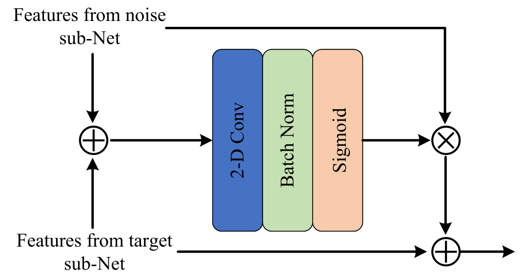
Fig. 8. Structure of the interaction module.
图8 交互模块的结构。
Features from the target subnet DTarget are first added to features from the noise subnet DNoise. Subsequently, we input the new features into a convolutional block consisting of a 2-D convolution layer, a BN layer, and a sigmoid activation function. A spectral mask M is produced and used to filter the information passed into the target subnet. Finally, the block adds DTarget and the filtered information to get the output features. The process of the interaction module is given by首先将来自目标子网D目标的特征添加到来自噪声子网D噪声的特征。随后,我们将新特征输入到由2-D卷积层,BN层和sigmoid激活函数组成的卷积块中。产生频谱掩码M并将其用于过滤传递到目标子网中的信息。最后,该模块将DTTarget和过滤后的信息相加以获得输出特征。交互模块的过程由下式给出: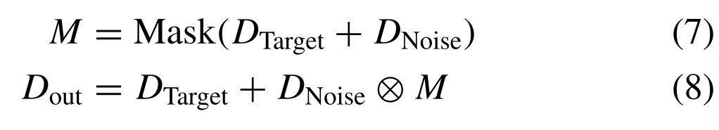
where ⊗ means elementwise multiplication and Mask(·) represents the shorthand for convolution, BN, and the sigmoid function. We will verify the effectiveness of the interaction module later in the ablation experiment.其中,⊗表示逐元素乘法,Mask(·)表示卷积、BN和sigmoid函数的简写。我们将在稍后的消融实验中验证交互模块的有效性。
D. Loss FunctionD.损失函数
Our proposed NAFSA-Net is designed to provide an accurate estimation of both noise and target audio at the same time. In this section, we modify the SI-SNR loss function to match the noise information and the target information from the two subnets. The weighted SI-SNR (wSI-SNR) loss function contains not only the original target estimation part SI-SNR(ˆs, s) but also the noise prediction term SI-SNR( ˆn, n)我们提出的NAFSA网络旨在同时提供噪声和目标音频的准确估计。在本节中,我们修改SI-SNR损失函数,以匹配来自两个SNR的噪声信息和目标信息。加权SI-SNR(wSI-SNR)损失函数不仅包含原始目标估计部分SI-SNR(ˆs, s),还包含噪声预测项SI-SNR( ˆn, n)
Although NAFSA-Net estimates both the noise and the target audio, the training of the model should still be dominated by the target audio. Therefore, we also propose an improved wSI-SNR (iwSI-SNR) loss function to guide the training of our model. The novel loss function increases the noise-aware perception component SI-SNR(x − ˆn, s). The iwSI-SNR loss is defined as虽然NAFSA-Net估计噪声和目标音频,但模型的训练仍然应该由目标音频主导。因此,我们还提出了一种改进的wSI-SNR(iwSI-SNR)损失函数来指导我们模型的训练。新的损失函数增加了噪声感知分量SI-SNR(x − ˆn, s)。iwSI-SNR损失定义为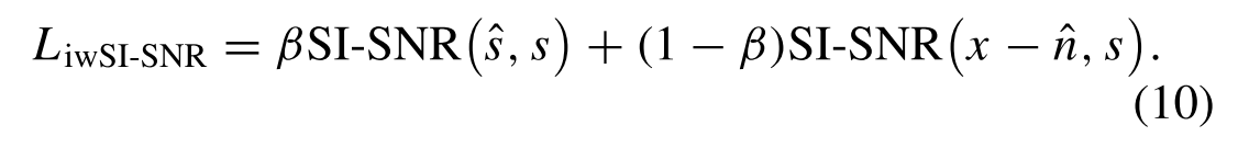
In the above equations, ˆn denotes the noise estimation. α and β are the weight factor, used for balancing the contribution of each loss part. In the experiments, we compared the denoising performance of the network when different loss functions are applied.在上述等式中,Wn表示噪声估计。α和β是权重因子,用于平衡每个损失部分的贡献。在实验中,我们比较了网络的去噪性能时,采用不同的损失函数。
IV. EXPERIMENTAL SETTINGS
四.实验设置
A. DatasetA.数据集
In our experiments, we trained and evaluated NAFSA-Net on ShipsEar [49], which is a public underwater acoustic signal dataset. We use two types of ship recordings (passengerboat and motorboat) and three types of underwater ambient noise signals (wind noise, flow noise, and rain noise) to generate the experimental dataset. The new dataset mixes ship signal with a randomly selected noise signal, synthesizing a total of 73 557 pieces of noisy audios with very low SNR range of [−15 dB, −5 dB], of which 70% are used for training, 20% for validation, and 10% for evaluation. For evaluation, we designed four different scenarios to perform NAFSA-Net: 1) seen ships, i.e., audios are from the same ships included in the training stage; 2) unseen ships, i.e., when signals are from the same ship types but different ships that are not included during training; 3) unseen ship types, i.e., when audios are from the unseen ship types (dredger and fishboat); and 4) unseen noise types, i.e., when audios are from the unseen noise types. The evaluation set is generated at three typical SNRs (−15, −10, and −5 dB). All noisy signals are resampled to 16 kHz and clipped to 3 s.在我们的实验中,我们在ShipsEar [49]上训练和评估了NAFSA-Net,这是一个公共的水声信号数据集。我们使用两种类型的船舶记录(快艇和摩托艇)和三种类型的水下环境噪声信号(风噪声,流噪声和雨噪声)来生成实验数据集。新数据集将船舶信号与随机选择的噪声信号混合,合成了总共73557段噪声音频,信噪比范围非常低,为[-15 dB,-5 dB],其中70%用于训练,20%用于验证,10%用于评估。为了进行评估,我们设计了四种不同的场景来执行NAFSA-Net:1)看到的船只,即,音频来自包括在训练阶段中的相同船只; 2)看不见的船只,即,当信号来自相同的船型但不同的船舶时,这些船舶在训练期间没有被包括在内; 3)看不见的船型,即,当音频来自看不见的船舶类型(挖泥船和渔船)时;以及4)看不见的噪声类型,即,当音频来自看不见的噪声类型时。评估集在三种典型SNR(−15、−10和−5 dB)下生成。所有噪声信号被重新采样到16 kHz并限幅到3 s。
B. Experiment DetailsB.实验细节
We set the window length of 32 ms (512 samples) and the frame shift of 16 ms (256 samples) to transform the waveform audios to the complex-valued spectrums. The Adam optimizer is used for optimization with an initial learning rate of 1e−4. The batch size is set to 32. In particular, the learning rate will decay by 0.9 if the evaluation of the validation set is not improved in two consecutive epochs. An early stopping mechanism is applied with a patience of 10 epochs. Our proposal is implemented by Pytorch and trained using NVIDIA A100 40-GB GPU.我们设置32 ms(512个样本)的窗口长度和16 ms(256个样本)的帧移位来将波形音频转换为复值频谱。Adam优化器用于初始学习率为1 e −4的优化。批量大小设置为32。特别地,如果验证集的评估在两个连续的时期中没有得到改善,则学习率将衰减0.9。一个早期停止机制是应用与耐心的10个时代。我们的建议是由Pytorch实现的,并使用NVIDIA A100 40-GB GPU进行训练。
C. Evaluation MetricsC.评估指标
To evaluate the performance of our proposals, we report the signal-to-distortion ratio (SDR) [50], scale-invariant SNR improvement (SI-SNRi), and segment SNR (SSNR) as objective metrics. Higher values correspond to better performance.为了评估我们的建议的性能,我们报告了信号失真比(SDR)[50],尺度不变SNR改善(SI-SNRi)和分段SNR(SSNR)作为客观指标。较高的值对应于较好的性能。
V. RESULTS AND DISCUSSIONS
五.成果和建议
A. Loss ComparisonsA.损失比较
In this section, we focus on the analysis of two different wSI-SNR loss functions and demonstrate the superiorities of our proposed iwSI-SNR in optimizing the noise-aware denoising network. In addition, we evaluate the performance of the setting of the weight factor in the loss function. Table I shows the performance of NAFSA-Net with different loss functions and different weight factors.在本节中,我们重点分析了两种不同的wSI-SNR损失函数,并展示了我们提出的iwSI-SNR在优化噪声感知去噪网络方面的优势。此外,我们评估的损失函数中的权重因子的设置的性能。表1显示了具有不同损失函数和不同权重因子的NAFSA网络的性能。
We first set the weight factors as the energy ratio of the target signal to the noise signal in [32] ($\alpha=|s|^2 /\left(|s|^2+|n|^2\right)$) to compare the performance of the two loss functions. It can be observed that iwSI-SNR evidently improves the SDR by 2.68 dB, the SI-SNRi by 0.88 dB, and the SSNR by 2.83 dB compared to wSI-SNR. This indicates that the iwSI-SNR loss function dominated by the target audio is more advantageous in model optimization. Next, we evaluate the effects of β in iwSI-SNR, which is set to {energy ratio, 0.3, 0.4, 0.5, 0.6, 0.7}. We can see that the performance on SI-SNR outperforms the case of β = energy ratio when β is set to a constant value. In addition, NAFSA-Net achieves optimal performance in each evaluation index when β = 0.5. These results demonstrate that the effectiveness of the proposed iwSI-SNR and the noise-aware term is equally important in improving the denoising performance compared with the target term.我们首先将权重因子设置为[32]中目标信号与噪声信号的能量比($\alpha=|s|^2 /\left(|s|^2+|n|^2\right)$)比较两种损失函数的性能。可以观察到,与wSI-SNR相比,iwSI-SNR明显地将SDR提高了2.68 dB,将SI-SNRi提高了0.88 dB,并且将SSNR提高了2.83 dB。这表明由目标音频主导的iwSI-SNR损失函数在模型优化中更有利。接下来,我们评估β在iwSI-SNR中的影响,其被设置为{能量比,0.3,0.4,0.5,0.6,0.7}。我们可以看到,当β设置为恒定值时,SI-SNR的性能优于β =能量比的情况。此外,当β = 0.5时,NAFSA-Net在各评价指标上均达到最优性能。这些结果表明,与目标项相比,所提出的iwSI-SNR和噪声感知项的有效性在改善去噪性能方面同样重要。
B. Parameter OptimizationB。参数优化
This section mainly optimizes the parameters w and d, which represents the window length and the number of adjacent time frames/frequency bins on each side of the subband attention module in the FSA block. In NAFSA-Net, we set d to be equal to w. To satisfy the fine-grained partitioning requirement, we set B to a small value of {2, 3, 4, 5, 6}. SDR, SI-SNRi, and SSNR scores for various models trained on the ShipsEar dataset are shown in Fig. 9. We observe that, for different w values, SI-SNRi results are similar. However, for both SDR and SSNR scores, the model achieved significantly better results than the other conditions when w = 4. Therefore, the subband width within the FSA block is set to w + 2d = 12.本节主要对参数w和d进行优化,参数w和d表示FSA块中子带注意模块每侧的窗口长度和相邻时间帧/频率仓的数量。在NAFSA网络中,我们将d设置为等于w。为了满足细粒度分区的要求,我们将B设置为一个小值{2,3,4,5,6}。在ShipsEar数据集上训练的各种模型的SDR、SI-SNRi和SSNR得分如图9所示。我们观察到,对于不同的w值,SI-SNRi结果是相似的。然而,对于SDR和SSNR评分,当w = 4时,该模型获得的结果显著优于其他条件。因此,FSA块内的子带宽度被设置为w + 2d = 12。
Fig. 9. Tuning the hyperparameter w.
见图9 调整超参数w。
C. Ablation StudyC.消融研究
In this section, we demonstrate the findings of ablation experiments performed to analyze the effectiveness of different network modules in our proposed NAFSA-Net. Four sets of comparison experiments are designed to evaluate the performance of different modules. First, we keep only one target subnet as the baseline, which is not estimated for noise. After that, the noise subnet is added to the baseline model, but there is no information interaction between the two subnets. Then, an interactive module is deployed between the target subnet and the noise subnet to obtain our proposed NAFSANet. Finally, we also evaluate the NAFSA-Net using the direct skip connection module. The first model uses the SI-SNR loss function, and the next three models utilize the iwSI-SNR loss function to optimize the training process. The results of the ablation study on the ShipsEar dataset are shown in Table II.在本节中,我们展示了消融实验的结果,以分析我们提出的NAFSA网络中不同网络模块的有效性。设计了四组对比实验来评估不同模块的性能。首先,我们只保留一个目标子网作为基线,这是没有估计的噪声。在此基础上,将噪声子网加入到基线模型中,但两个子网之间没有信息交互。然后,在目标子网和噪声子网之间部署交互模块,以获得我们提出的NAFSANet。最后,我们还评估了NAFSA网络使用直接跳过连接模块。第一个模型使用SI-SNR损失函数,接下来的三个模型使用iwSI-SNR损失函数来优化训练过程。ShipsEar数据集上的消融研究结果如表II所示。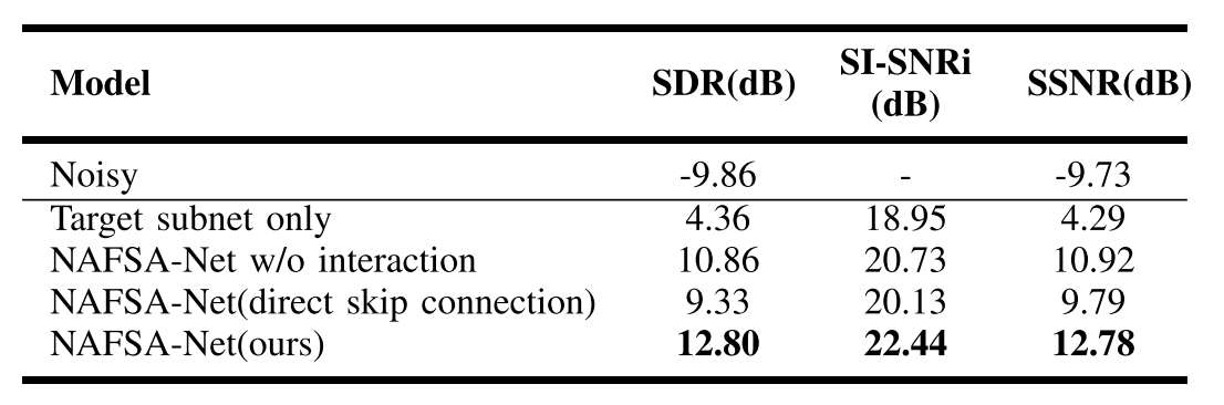
TABLE II ABLATION STUDY ON THE SHIPSEAR DATASET
表二:船舶数据集上的烧蚀研究
We can see from Table II that the single target subnet improves the SDR by 14.22 dB, SISNR by 18.95 dB, and SSNR by 14.02 dB compared to the noisy audio. After adding the noise estimation subnet, we observe a 6.5-dB gain on SDR, 1.68-dB gain on SI-SNRi, and 6.63-dB gain on SSNR. When the information interaction module is introduced to the network, NAFSA-Net achieves further 1.94-, 1.71-, and 1.86-dB improvements in SDR, SI-SNRi, and SSNR, respectively. In addition, we further evaluate the effectiveness of gated convolution in the skip connection module. Our method achieves a gain on SDR by 3.47 dB, SI-SNRi by 2.31 dB, and SSNR by 2.99 dB, compared with the direct skip connection module. Since both subnets share the same encoder part, NAFSA-Net can filter valuable information through gated convolutional connections and transmit them to both subnets separately. These observations verify the effectiveness of the proposed noise-aware network architecture, the interaction module, and the gated convolution connection for enhancing the denoising capability in the case of low SNR.从表II中可以看出,与噪声音频相比,单个目标子网将SDR提高了14.22 dB,将SISNR提高了18.95 dB,将SSNR提高了14.02 dB。添加噪声估计子网后,SDR上的增益为6.5 dB,SI-SNRi上的增益为1.68 dB,SSNR上的增益为6.63 dB。当将信息交互模块引入网络时,NAFSA-Net在SDR、SI-SNRi和SSNR方面分别实现了1.94、1.71和1.86 dB的改进。此外,我们进一步评估了门控卷积在跳过连接模块中的有效性。与直接跳过连接模块相比,我们的方法在SDR上实现了3.47 dB的增益,SI-SNRi为2.31 dB,SSNR为2.99 dB。由于这两个编码器共享相同的编码器部分,NAFSA-Net可以通过门控卷积连接过滤有价值的信息,并将它们分别传输到两个编码器。这些观察结果验证了所提出的噪声感知网络架构、交互模块和门控卷积连接在低SNR情况下增强去噪能力的有效性。
D. Comparison With BaselinesD.与基线的比较
In this section, we analyze the results to show the advantages of NAFSA-Net over previous techniques in terms of denoising. As a comparison, a wavelet threshold shrinking denoising method and an EMD method are used for the conventional baseline models. The level of wavelet decomposition is set to be $\left\lfloor\log _2(L) / 2\right\rfloor$, where L is the number of sample points. The EMD approach follows the setting of [11]. In addition, we further compare NAFSA-Net with other representative DNN-based approaches, which are briefly introduced as follows.在本节中,我们将分析结果,以显示NAFSA-Net在去噪方面优于以前的技术。作为比较,小波阈值收缩去噪方法和EMD方法被用于常规基线模型。小波分解的水平被设置为$\left\lfloor\log _2(L) / 2\right\rfloor$,其中L是样本点的数量。EMD方法遵循[11]的设置。此外,我们还将NAFSA-Net与其他代表性的基于DNN的方法进行了比较,简要介绍如下。
1)SEGAN: A time-domain enhancement approach with the generative adversarial network (GAN).
2)DPRNN for Denoising: A dual-path recurrent neural network in the time domain.
3)DCCRN: A T-F domain complex-valued denoising model.
4)FullSubNet: A T-F domain method that aggregates the fullband features and the subband features to enhance the denoising performance.
5)NAFSA-Fullband: NAFSA-Net with only fullband attention in the FSA blocks.
6)NAFSA-Subband: NAFSA-Net with only subband attention module in the FSA blocks.1)SEGAN:一种使用生成对抗网络(GAN)的时域增强方法。2)DPRNN for Denoising:时域中的双路径递归神经网络。3)DCCRN:一种T-F域复值去噪模型。4)FullSubNet:一种T-F域方法,聚合全带特征和子带特征以增强去噪性能。5)NAFSA-全波段:NAFSA-网络,仅在FSA块中关注全波段。6)NAFSA-子带:在FSA块中仅具有子带注意模块的NAFSA-网络。
All the above models are trained on the same ShipsEar dataset for 100 epochs.所有上述模型都在相同的ShipsEar数据集上训练了100个epochs。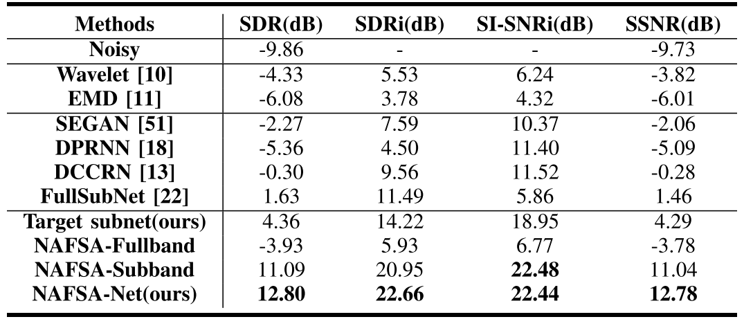
TABLE III QUANTITATIVE COMPARISONS WITH OTHER DENOISING METHODS ON THE SHIPSEAR DATASET
表三:与船舶数据集上其他降噪方法的定量比较
The overall results on SDR, SDRi, SI-SNRi, and SSNR are shown in Table III. First, we find that the traditional statistical-based techniques perform poorly for processing underwater acoustic signals with low SNRs, and the DNN-based denoising methods outperform the conventional denoising approach DNN-based denoising methods outperform the conventional denoising approaches in all evaluation metrics. Besides, our proposed NAFSA-Net (last row) achieves the best evaluation scores on the ShipsEar dataset, considerably better than other models. NAFSA-Net obtains a 22.66-dB gain on SDR, a 22.44-dB gain on SI-SNR, and a 22.51-dB gain on SSNR. In addition, we can see that the single target subnet with FSA blocks shows a very competitive denoising performance and achieves the best results among all methods based on target audio estimation. This result demonstrates that the FSA blocks proposed in this article can effectively extract the features of the target audio from the low SNR noisy signals. We have further evaluated the role of the fullband module and the subband module in the NAFSA-Net. The fine-grained subband model shows a greater advantage in denoising, and it obtains a similar SI-SNRi score as NAFS DNN-based denoising methods outperform the conventional denoising approaches in all evaluation metrics. Besides, our proposed NAFSA-Net (last row) achieves the best evaluation scores on the ShipsEar dataset, considerably better than other models. NAFSA-Net obtains a 22.66-dB gain on SDR, a 22.44-dB gain on SI-SNR, and a 22.51-dB gain on SSNR. In addition, we can see that the single target subnet with FSA blocks shows a very competitive denoising performance and achieves the best results among all methods based on target audio estimation. This result demonstrates that the FSA blocks proposed in this article can effectively extract the features of the target audio from the low SNR noisy signals. We have further evaluated the role of the fullband module and the subband module in the NAFSA-Net. The fine-grained subband model shows a greater advantage in denoising, and it obtains a similar SI-SNRi score as NAFSA-Net. It is expected that properly aggregating the long-term fullband and the fine-grained subband can further improve the denoising performance of our model. Table IV presents the experimental results of our proposed NAFSA-Net at different SNRs. One can observe that NAFSA-Net can restore the noisy signals to the same level for different SNR conditions (i.e. recover from −5, −10, and −15 dB to 12.65, 13.24, and 10.39 dB, respectively). These suggest that, even in the case of low SNRs, NAFSA-Net is an effective solution to model the characteristics of the target ships, so as to realize underwater acoustic denoising.SDR、SDRi、SI-SNRi和SSNR的总体结果见表III。首先,我们发现传统的基于神经网络的技术在处理低信噪比的水声信号时表现不佳,基于DNN的去噪方法优于传统的去噪方法。此外,我们提出的NAFSA-Net(最后一行)在ShipsEar数据集上获得了最佳评估分数,比其他模型要好得多。NAFSA-Net在SDR上获得22.66 dB增益,在SI-SNR上获得22.44 dB增益,在SSNR上获得22.51 dB增益。此外,我们可以看到,具有FSA块的单个目标子网显示出非常有竞争力的去噪性能,并且在所有基于目标音频估计的方法中达到了最好的结果。实验结果表明,本文提出的FSA模块可以有效地从低信噪比噪声信号中提取目标音频的特征。我们进一步评估了全带模块和子带模块在NAFSA网络中的作用。细粒度子带模型在去噪方面表现出更大的优势,并且它获得了与NAFS DNN去噪方法相似的SI-SNRi得分,在所有评价指标上都优于传统的去噪方法。此外,我们提出的NAFSA-Net(最后一行)在ShipsEar数据集上获得了最佳评估分数,比其他模型要好得多。NAFSA-Net在SDR上获得22.66 dB增益,在SI-SNR上获得22.44 dB增益,在SSNR上获得22.51 dB增益。此外,我们可以看到,具有FSA块的单个目标子网显示出非常有竞争力的去噪性能,并且在所有基于目标音频估计的方法中达到了最好的结果。实验结果表明,本文提出的FSA模块可以有效地从低信噪比噪声信号中提取目标音频的特征。我们进一步评估了全带模块和子带模块在NAFSA网络中的作用。细粒度子带模型在去噪方面表现出更大的优势,并且它获得了与NAFSA-Net相似的SI-SNRi得分。可以预期,适当地聚合长期全频带和细粒度子带可以进一步提高我们的模型的去噪性能。表IV给出了我们提出的NAFSA-Net在不同SNR下的实验结果。可以观察到,NAFSA-Net可以在不同的SNR条件下将噪声信号恢复到相同的水平(即分别从−5、−10和−15 dB恢复到12.65、13.24和10.39 dB)。这表明,即使在低信噪比的情况下,NAFSA网络是一个有效的解决方案来建模的目标船舶的特性,从而实现水声降噪。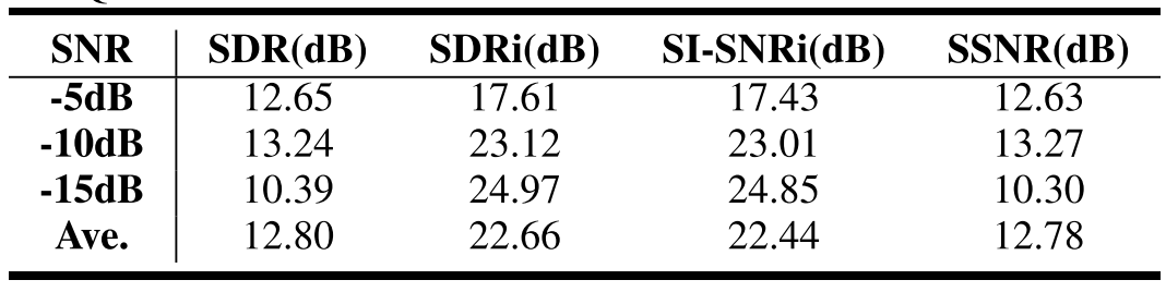
TABLE IV QUANTITATIVE RESULTS OF NAFSA-NET AT DIFFERENT SNRS
表IV不同信噪比下NAFSA网络的定量结果
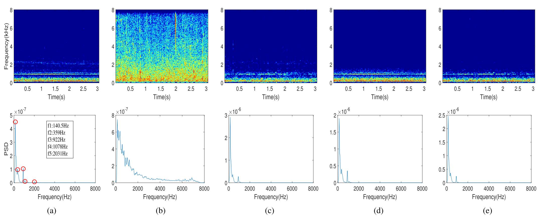
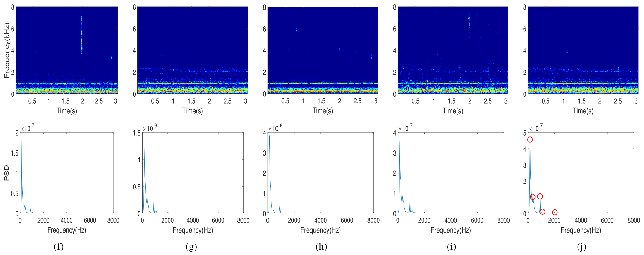
Fig. 10. Comparison of the T-F magnitudes and PSD of motorboat audio processed using DNN-based techniques. (a) Clean. (b) Noisy. (c) SEGAN. (d) DPRNN. (e) DCCRN. (f) FullSubNet. (g) Target subnet. (h) NAFSA-Fullband. (i) NAFSA-Subband. (j) NAFSA-Net(ours).
见图10。使用基于DNN的技术处理的摩托艇音频的T-F幅度和PSD的比较。(a)干净(b)吵了.(c)塞甘(d)DPRNN。(e)DCCRN。(f)全子网(g)目标子网。(h)NAFSA-全波段。(i)NAFSA-子带。(j)NAFSA网络(我们的)。
To explore the denoising performance of our proposed NAFSA-Net, we further compare the denoising differences of noisy audio of motorboats in diverse DNN-based techniques. Fig. 10 demonstrates the magnitude and PSD of the clean audio, the noisy audio, and the denoised audio processed by different DNN-based methods. It can be observed from Fig. 10(j) that our proposed NAFSA-Net shows substantial superiority in noise suppression and clean signal restoration. The clean motorboat audio consists of five dominant frequencies, which are 140.5, 359, 922, 1078, and 2031 Hz, respectively. NAFSA-Net fully recovers both low-frequency components with high fidelity and the low-energy components distributed in the high-frequency part. In comparison with SEGAN, DPRNN, DCCRN, and FullSubNet, they are unable to exactly recover the original clean signal. In these methods, the weak-energy frequency components (1078 and 2031 Hz) distributed in the high-frequency part are eliminated as noise, resulting in distortion of the denoised signals. Fig. 10(g) shows the results of a single target subnet, which aggregates advantages of both long-range dependencies and short-term correlations of spectral features through the FSA block. This method retrains a small number of noise components but is still superior in suppressing underwater ambient noise compared to the previous DNN-based methods. As for the NAFSA-fullband model and the NAFSA-subband model, the former focuses on the overall structure of the spectrogram and tends to ignore the small variations of the motorboat audio. NAFSANet combines the advantages of both fullband and subband models while training the target estimation subnet with the aid of a noise prediction subnet. Our proposals accurately separate the target signal from the noisy audio with less distortion.为了探索我们提出的NAFSA网络的去噪性能,我们进一步比较了不同基于DNN的技术中摩托艇噪声音频的去噪差异。图10展示了通过不同的基于DNN的方法处理的干净音频、有噪音频和去噪音频的幅度和PSD。从图10(j)可以看出,我们提出的NAFSA-Net在噪声抑制和干净信号恢复方面表现出显著的优越性。干净的摩托艇音频由五个主频组成,分别为140.5、359、922、1078和2031 Hz。NAFSA-Net完全恢复具有高保真度的低频分量和分布在高频部分的低能量分量。与SEGAN、DPRNN、DCCRN和FullSubNet相比,它们无法准确地恢复原始的干净信号。在这些方法中,分布在高频部分的弱能量频率分量(1078和2031 Hz)作为噪声被消除,导致去噪信号的失真。图10(g)示出了单个目标子网的结果,其通过FSA块聚合了频谱特征的长期依赖性和短期相关性两者的优点。该方法抑制了少量的噪声分量,但与以前的基于DNN的方法相比,在抑制水下环境噪声方面仍然具有上级优势。至于NAFSA-全频带模型和NAFSA-子带模型,前者关注频谱图的整体结构,往往忽略摩托艇音频的微小变化。NAFSANet结合了全带和子带模型的优点,同时在噪声预测子网的帮助下训练目标估计子网。我们的建议准确地分离目标信号从嘈杂的音频失真较小。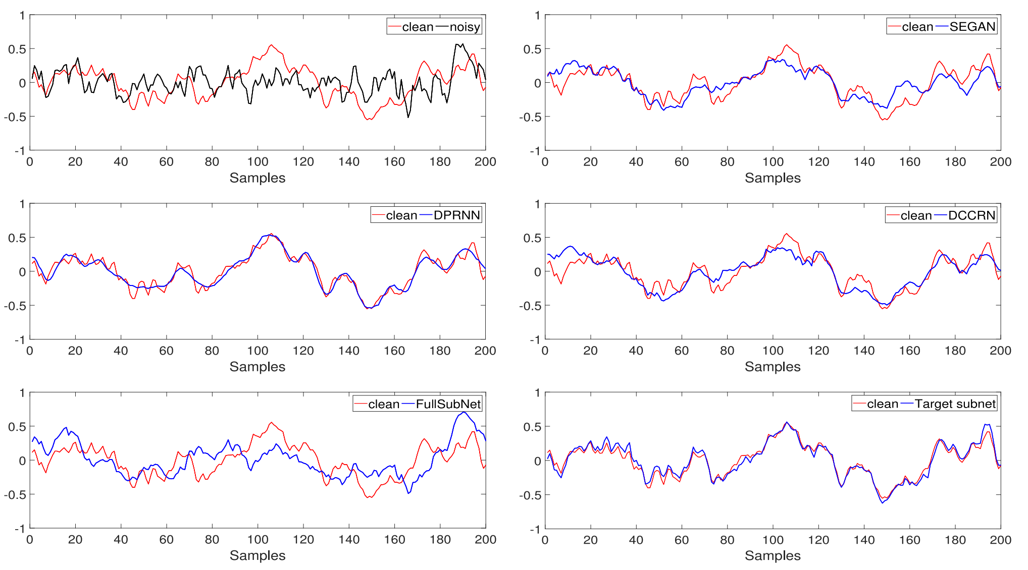
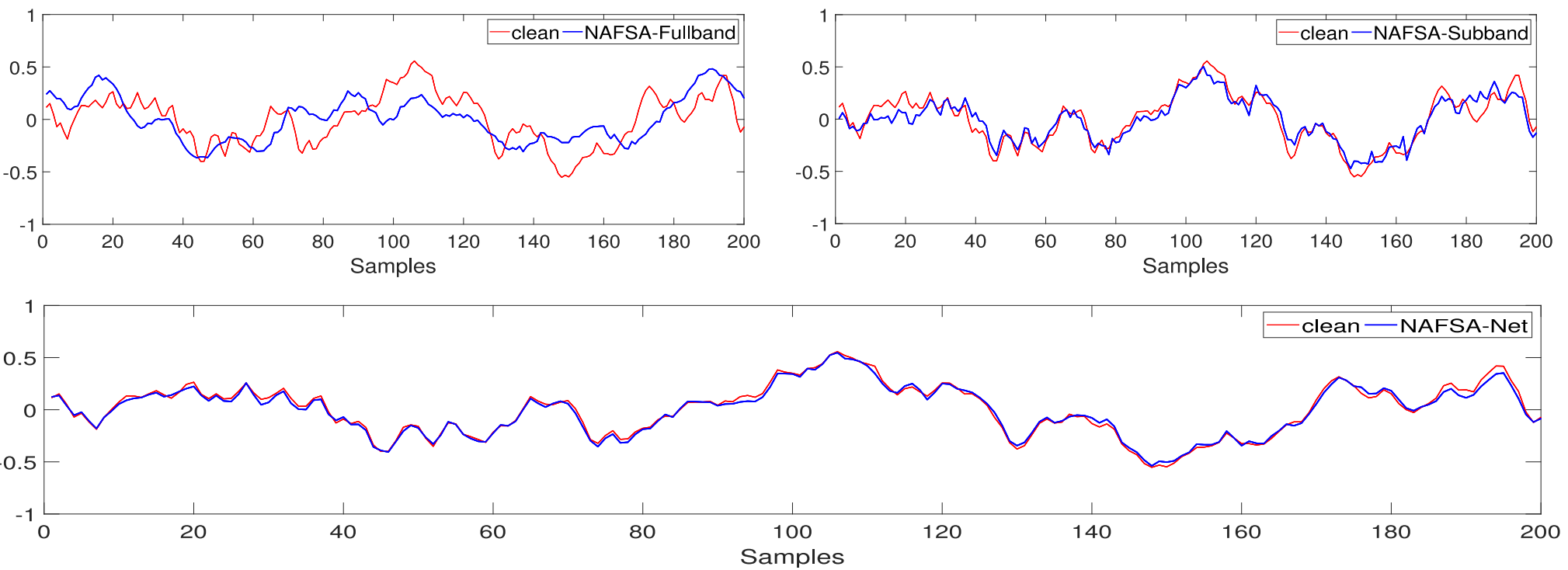
Fig. 11. Illustration of the reference target audio with the denoised audio by DNN-based methods in the time domain.
见图11。参考目标音频与时域中基于DNN方法的去噪音频的图示。
The time-domain representations of denoised signals by different DNN-based approaches are shown in Fig. 11, in which red lines indicate the reference ship audios, the black line represents the corrupted signal by underwater background noise, and blue lines correspond to denoised vessel audios by diverse DNN-based methods. In the corrupted signals with low SNRs, the spectral characteristics of target audio are completely masked by the noise, especially the weak-energy high-frequency spectral components [see Fig. 10(b)]. Although the previous techniques, such as SEGAN, DPRNN, DCCRN, and FullSubNet, outperform the conventional methods in terms of denoising performance, they fail to follow subtle variations in the high-frequency part. As a comparison, the estimated audios by our proposed single target subnet and NAFSA-subband models are in better agreement with the clean audio waveform. They capture some of the small details of the high-frequency components in the target signals. However, even so, we also find that the audio estimated by these two methods still does not match the original audio perfectly due to the presence of noise-like components in the vessel signals. Finally, we can confirm that our proposed NAFSA-Net handles the aforementioned problems, and the denoised audio is well-aligned with the reference signal.图11中示出了通过不同的基于DNN的方法进行去噪的信号的时域表示,其中红线表示参考船舶音频,黑线表示被水下背景噪声破坏的信号,蓝线对应于通过不同的基于DNN的方法进行去噪的船舶音频。在低信噪比的受损信号中,目标音频的频谱特征完全被噪声掩盖,特别是弱能量的高频频谱分量[见图10(b)]。虽然以前的技术,如SEGAN,DPRNN,DCCRN和FullSubNet,在去噪性能方面优于传统方法,但它们无法跟踪高频部分的细微变化。作为比较,我们提出的单目标子网和NAFSA子带模型的估计音频与干净的音频波形更好地吻合。它们捕获目标信号中高频分量的一些小细节。然而,即使如此,我们也发现,这两种方法估计的音频仍然不匹配的原始音频完美,由于在血管信号中的噪声样成分的存在。最后,我们可以确认我们提出的NAFSA网络处理了上述问题,并且去噪音频与参考信号对齐良好。
E. Evaluation on Unseen DatasetsE.对未知数据集的评估
This section further explores the generalization performance of our proposed NAFSA-Net on unseen datasets. For this purpose, we design three different unseen scenarios to test our proposals. The first is the scenario of unseen ships, in which the types of ships are the same as those in the training dataset (passengerboat and motorboat), but from different ships. The second is the unseen ship types dataset, which consists of noisy audio from new vessel types (fishboat and dredger). As for the unseen noise scenario, we generate the test dataset by mixing the noise signals collected from other seas (the South China Sea) with the ship signals from ShipsEar. Fig. 12 presents the experimental results of our proposed NAFSA-Net on three different unseen datasets.本节进一步探讨了我们提出的NAFSA-Net在看不见的数据集上的泛化性能。为此,我们设计了三个不同的看不见的场景来测试我们的建议。第一种是看不见的船只场景,其中船只的类型与训练数据集中的船只相同(快艇和摩托艇),但来自不同的船只。第二个是看不见的船舶类型数据集,其中包括来自新船舶类型(渔船和挖泥船)的嘈杂音频。对于看不见的噪声场景,我们通过将从其他海域(南中国海)收集的噪声信号与ShipsEar的船舶信号混合来生成测试数据集。图12展示了我们提出的NAFSA网络在三个不同的看不见的数据集上的实验结果。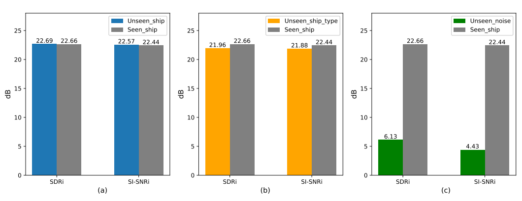
Fig. 12. Evaluation of proposed NAFSA-Net for unseen datasets in terms of SDRi and SI-SNRi. (a) Unseen ship. (b) Unseen_ship_type. (c) Unseen_noise.
见图12 根据SDRi和SI-SNRi评估拟议的NAFSA-Net用于看不见的数据集。(a)看不见的船(b)Unseen_ship_type.(c)看不见的噪音。
For the unseen ship dataset [see Fig. 12(a)], we can observe that the denoising performance of our proposed NAFSA-Net is not affected. It achieves similar SDRi and SI-SNRi scores on the new dataset as before. Besides, for the unseen ship type dataset [see Fig. 12(b)], NAFSA-Net improves SDRi by an average of 21.96 dB and SI-SNRi by an average of 21.88 dB on the output results. Different ships, especially when they are from different types, tend to demonstrate unique spectral characteristics, but the performance of NAFSA-Net only marginally degrades the SDRi by 3.1% and SI-SNRi by 2.5% on the unseen ship types dataset. The results of the spectrum analysis of the unseen ship example and unseen ship type example are shown in Figs. 13 and 14, respectively. Nonetheless, for the unseen noise dataset [see Fig. 12(c)], the results processed by the model showed a slight improvement in each metric compared to the original noisy signals. One possible reason is that the noise samples (rain, flow, and wind) in the ShipsEar dataset are collected from the sea surface, while the comparison noise samples are taken from the underwater environment. There are major differences in the spectral characteristics of the noise in the two environments. All the above results suggest that our proposed model is able to effectively deal with unseen data with similar noise features while generalizing poorly on the unseen noise dataset.对于看不见的船舶数据集[见图12(a)],我们可以观察到我们提出的NAFSA-Net的去噪性能不受影响。它在新数据集上实现了与以前类似的SDRi和SI-SNRi分数。此外,对于不可见的船型数据集[见图12(b)],NAFSA-Net在输出结果上将SDRi平均提高了21.96 dB,将SI-SNRi平均提高了21.88 dB。不同的船舶,特别是来自不同类型的船舶,往往会表现出独特的光谱特征,但NAFSA-Net的性能在看不见的船舶类型数据集上仅使SDRi降低3.1%,SI-SNRi降低2.5%。未看见船舶实例和未看见船型实例的频谱分析结果示于图1和图2中。分别为13和14。尽管如此,对于看不见的噪声数据集[见图12(c)],与原始噪声信号相比,模型处理的结果显示每个度量都略有改善。一个可能的原因是ShipsEar数据集中的噪声样本(雨、流和风)是从海面收集的,而比较噪声样本是从水下环境中采集的。在两种环境中噪声的频谱特性有很大差异。所有上述结果表明,我们提出的模型能够有效地处理具有相似噪声特征的不可见数据,而在不可见噪声数据集上的泛化能力较差。
Fig. 13. T-F magnitude and PSD of clean audio, noisy audio, and denoised audio for an unseen ship (passengerboat). (a) Magnitude spectra of the clean signal. (b) PSD of the clean signal. (c) Magnitude spectra of the noisy signal. (d) PSD of the noisy signal. (e) Magnitude spectra of the denoised signal. (f) PSD of the denoised signal.
图13.一艘看不见的船(快艇)的干净音频、嘈杂音频和去噪音频的T-F幅度和PSD。(a)干净信号的幅度谱。(b)干净信号的PSD。(c)噪声信号的幅度谱。(d)噪声信号的PSD。(e)去噪信号的幅度谱。(f)去噪信号的PSD。
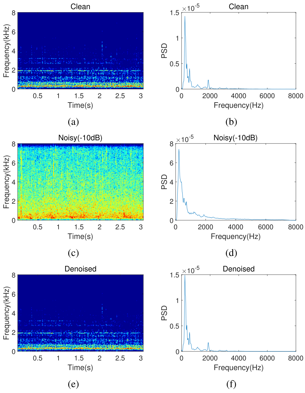
Fig. 14. T-F magnitude and PSD of clean audio, noisy audio, and denoised audio for an unseen ship type sample (fishboat). (a) Magnitude spectra of the clean signal. (b) PSD of the clean signal. (c) Magnitude spectra of the noisy signal. (d) PSD of the noisy signal. (e) Magnitude spectra of the denoised signal. (f) PSD of the denoised signal.
见图14。对于看不见的船型样本(渔船),干净音频、嘈杂音频和去噪音频的T-F幅度和PSD。(a)干净信号的幅度谱。(b)干净信号的PSD。(c)噪声信号的幅度谱。(d)噪声信号的PSD。(e)去噪信号的幅度谱。(f)去噪信号的PSD。
F. Preliminary Exploration on Unseen Noise DatasetF.不可见噪声数据集初探
Section V-E points out that the denoising performance degrades significantly when the trained NAFSA-Net is directly applied to the new noise dataset. In light of this, we have purposefully explored some possible solutions. From the previous analysis, we know that NAFSA-Net shows good generalization for unknown target ship datasets. Therefore, a straightforward approach is to construct a new dataset using existing ship data and noise data from the target sea area and retrain the model on the new dataset. In addition, we can use a small number of samples from the target sea to fine-tune our pretrained NAFSA-Net. To verify the effectiveness of the two methods, we construct two datasets using the noise signals from the South China Sea and the ship signals from the ShipsEar dataset. These two datasets contain 21 313 noisy audios with SNRs in the range of [−15 dB, −5 dB] and [−20 dB, 10 dB], respectively. All noisy audios are resampled to 16 kHz and clipped to 3 s. Table V shows the experimental results of the two schemes on the unseen noise dataset.第V-E节指出,当训练好的NAFSA-Net直接应用于新的噪声数据集时,去噪性能会显着下降。有鉴于此,我们有目的地探索了一些可能的解决方案。从前面的分析中,我们知道NAFSA网络对未知目标船数据集表现出良好的泛化能力。因此,一种直接的方法是使用来自目标海域的现有船舶数据和噪声数据构建新的数据集,并在新的数据集上重新训练模型。此外,我们可以使用来自目标海域的少量样本来微调预训练的NAFSA网络。为了验证这两种方法的有效性,我们使用来自南海的噪声信号和来自ShipsEar数据集的船舶信号构建了两个数据集。这两个数据集包含21313个噪声音频,SNR分别在[−15 dB,−5 dB]和[−20 dB,10 dB]范围内。所有嘈杂的音频都被重新采样到16 kHz,并被限幅到3 s。表V显示了两种方案在不可见噪声数据集上的实验结果。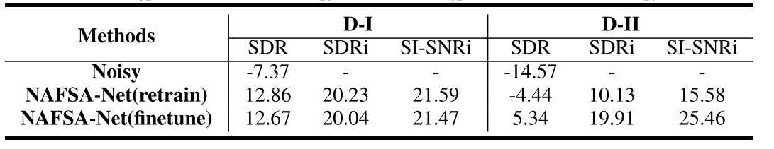
TABLE V QUANTITATIVE COMPARISONS OF NAFSA-NET ON UNSEEN DATASETS D-I ([−15 DB, −5 DB]) AND D-II ([−20 DB, −10 DB])
表V NAFSA-NET在未观测数据集D-I([-15 DB,-5 DB])和D-II([-20 DB,-10 DB])上的定量比较
We first evaluate our proposed NAFSA-Net on the D-I dataset. As shown in Table V, “NAFSA-Net(retrain)” and “NAFSA-Net(finetune)” achieve similar results on each evaluation metric. Compared to the original noisy audios, these two schemes improve the SDR by an average of 20.13 dB and SI-SNR by an average of 21.53 dB. These results demonstrate that both solutions are effective for handling unseen noise datasets with an SNR range of [−15 dB, −5 dB]. When it comes to the dataset with lower SNR, we can observe that the retraining approach achieves a mere 10.13-dB gain on SDR and 25.58-dB gain on SI-SNR. As a comparison, the fine-tuning method further improves the SDR and SISNR scores by 9.78 and 9.88 dB compared to the former. These analyses point out that both the retraining method and the fine-tuning scheme can effectively address the adaptation of the model to an unseen noise dataset, while the fine-tuning scheme shows greater potential for improving the denoising performance of our model in low SNR conditions.我们首先在D-I数据集上评估我们提出的NAFSA网络。如表V所示,“NAFSA-Net(retrain)”和“NAFSA-Net(finetune)”在每个评价指标上实现了类似的结果。与原始噪声音频相比,这两种方案平均提高了20.13 dB的SDR和21.53 dB的SI-SNR。这些结果表明,这两种解决方案都能有效处理SNR范围为[−15 dB,−5 dB]的不可见噪声数据集。当涉及到具有较低SNR的数据集时,我们可以观察到再训练方法在SDR上仅实现了10.13 dB增益,在SI-SNR上仅实现了25.58 dB增益。作为比较,与前者相比,微调方法进一步将SDR和SISNR分数提高了9.78和9.88 dB。这些分析指出,再训练方法和微调方案都可以有效地解决模型对不可见噪声数据集的适应问题,而微调方案在低信噪比条件下提高模型的去噪性能方面具有更大的潜力。
VI. CONCLUSION
六.结论
In this article, a novel NAFSA-Net is introduced for underwater acoustic signal denoising in the case of extremely low SNR. This solution uses different subnets to estimate both the noise and the target audio, and the noise subnet is designed to assist in the training of the target subnet. We have trained NAFSA-Net on the seen and unseen datasets generated by real ship signals and underwater ambient noise signals. Experimental results have illustrated the superiority over conventional methods and DNN-based denoising approaches.本文提出了一种新的NAFSA网络,用于极低信噪比情况下的水声信号去噪。该解决方案使用不同的带宽来估计噪声和目标音频,并且噪声子网被设计为辅助目标子网的训练。我们已经在由真实的船舶信号和水下环境噪声信号生成的可见和不可见数据集上训练了NAFSA-Net。实验结果表明,该方法优于传统方法和基于DNN的去噪方法。
We have found that the noise-aware learning method can substantially improve the ability of handling underwater acoustic signals with very low SNRs. Compared with the single target subnet, NAFSA-Net achieves a 59.35% gain on SDRi and an 18.42% gain on SI-SNRi. Furthermore, we have evaluated different feature extraction strategies, i.e., single fullband attention, single subband attention, and FSA, and found that a combination of fullband attention and subband attention shows great advantages in extracting features of underwater acoustic audios. In addition, we have trained NAFSA-Net with two different wSI-SNR loss functions. Our proposed iwSI-SNR loss function is guided by the target audio and integrates the output information of both subnets, which shows greater potential in optimizing the training of our model. Under the same setting conditions, the iwSI-SNR loss function helps NAFSA-Net improve the SDR by 2.68 dB, the SI-SNRi by 0.88 dB, and the SSNR by 2.77 dB compared with the wSI-SNR loss function.我们已经发现,噪声感知学习方法可以大大提高处理非常低的信噪比的水声信号的能力。与单一目标子网相比,NAFSA-Net在SDRi上获得了59.35%的增益,在SI-SNRi上获得了18.42%的增益。此外,我们还评估了不同的特征提取策略,即,单全带注意、单子带注意和FSA的研究结果表明,全带注意和子带注意相结合的方法在提取水声音频特征方面具有很大的优势。此外,我们还使用两种不同的wSI-SNR损失函数训练了NAFSA-Net。我们提出的iwSI-SNR损失函数由目标音频引导,并整合了两个音频的输出信息,这在优化我们模型的训练方面显示出更大的潜力。在相同的设置条件下,与wSI-SNR损失函数相比,iwSI-SNR损失函数帮助NAFSA-Net将SDR提高了2.68 dB,SI-SNRi提高了0.88 dB,SSNR提高了2.77 dB。
We have evaluated NAFSA-Net against three different unseen datasets. Experimental results show that our proposed NAFSA-Net has good generalization for unseen target ship audios. However, the denoising performance of the model degrades significantly in the unseen noise dataset. To this end, we further explored possible solutions to the problem of adaptation to unseen noise datasets. Therefore, a future research direction could be optimizing the generalization of the model in different noise environments and exploring the possibilities of using the same model to process different marine environmental data.我们已经针对三个不同的看不见的数据集对NAFSA网络进行了评估。实验结果表明,我们提出的NAFSA网络具有良好的泛化能力,不可见的目标船舶音频。然而,该模型的去噪性能在不可见的噪声数据集中显着下降。为此,我们进一步探索了适应不可见噪声数据集问题的可能解决方案。因此,优化模型在不同噪声环境下的泛化能力,探索用同一模型处理不同海洋环境数据的可能性,是未来的研究方向。